Econometrics I Professor William Greene Stern School of

Econometrics I Professor William Greene Stern School of Business Department of Economics 10 -/39 Part 10: Interval Estimation

Econometrics I Part 10 – Interval Estimation and Prediction 10 -/39 Part 10: Interval Estimation

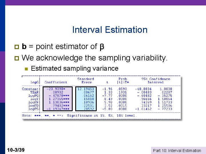
Interval Estimation b = point estimator of p We acknowledge the sampling variability. p n n 10 -3/39 Estimated sampling variance b = + sampling variability induced by Part 10: Interval Estimation

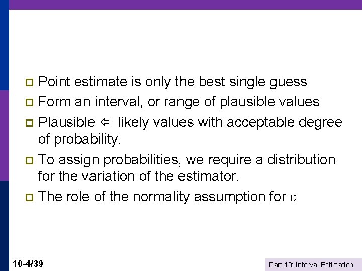
Point estimate is only the best single guess p Form an interval, or range of plausible values p Plausible likely values with acceptable degree of probability. p To assign probabilities, we require a distribution for the variation of the estimator. p The role of the normality assumption for p 10 -4/39 Part 10: Interval Estimation

Robust Inference: Confidence Interval for βk bk = the point estimate Std. Err[bk] = sqr{Estimated Asymptotic Variance of bk} = vk The matrix may be any robust or appropriate covariance matrix. n bk ~ Asy. N[βk, vk 2] n (bk-βk)/vk ~ Asy. N[0, 1] Consider a range of plausible values of βk given the point estimate bk. bk sampling error. n n n 10 -5/39 Measured in standard error units, |(bk – βk)/ vk| < z* Larger z* greater probability (“confidence”) Given normality, e. g. , z* = 1. 96 95%, z*=1. 645 90% Plausible range for βk then is bk ± z* vk Part 10: Interval Estimation

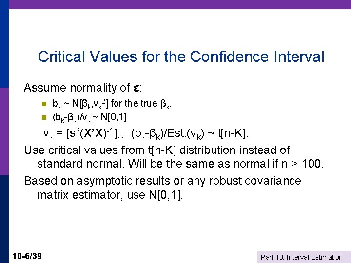
Critical Values for the Confidence Interval Assume normality of ε: n n bk ~ N[βk, vk 2] for the true βk. (bk-βk)/vk ~ N[0, 1] vk = [s 2(X’X)-1]kk (bk-βk)/Est. (vk) ~ t[n-K]. Use critical values from t[n-K] distribution instead of standard normal. Will be the same as normal if n > 100. Based on asymptotic results or any robust covariance matrix estimator, use N[0, 1]. 10 -6/39 Part 10: Interval Estimation

Confidence Interval Critical t[. 975, 29] = 2. 045 Confidence interval based on t: 1. 27365 2. 045 *. 1501 Confidence interval based on normal: 1. 27365 1. 960 *. 1501 10 -7/39 Part 10: Interval Estimation

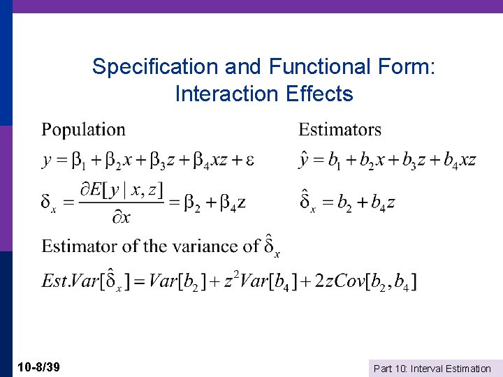
Specification and Functional Form: Interaction Effects 10 -8/39 Part 10: Interval Estimation

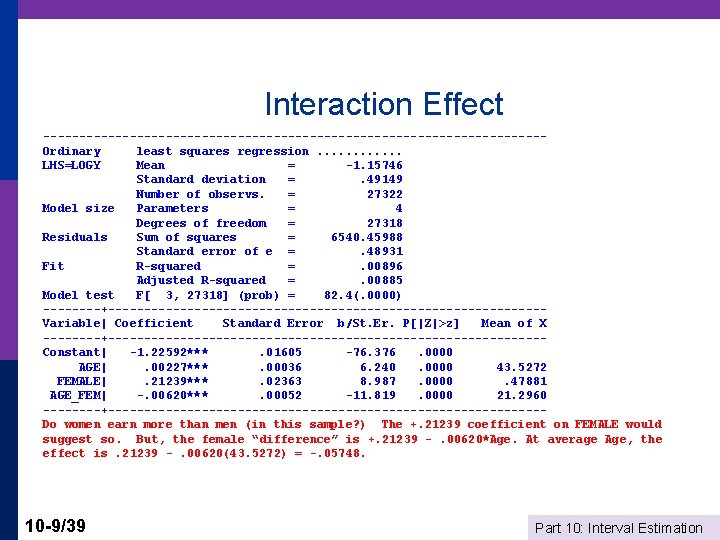
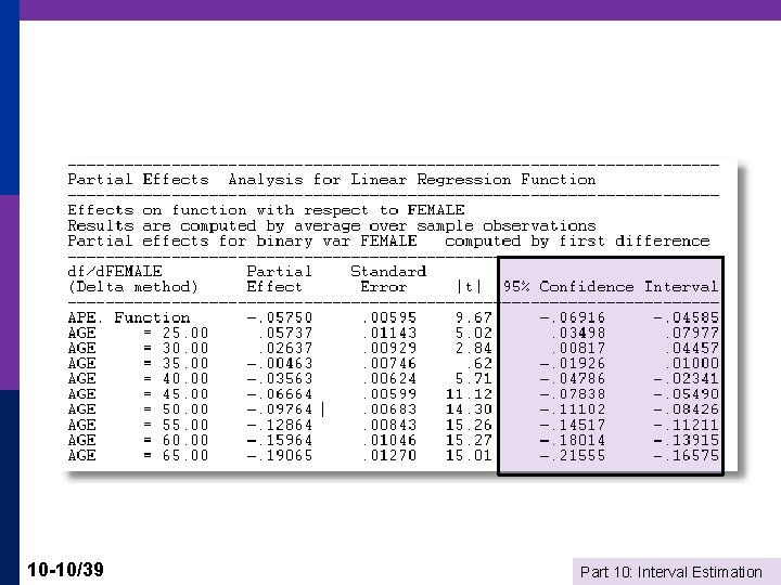
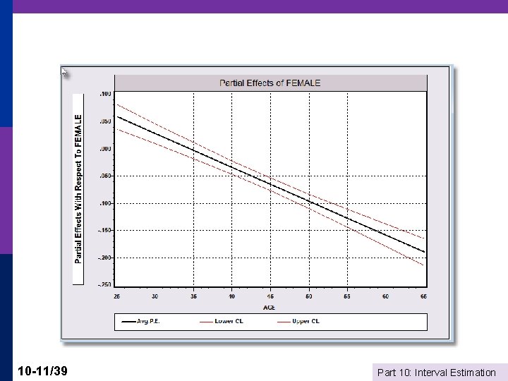
Interaction Effect -----------------------------------Ordinary least squares regression. . . LHS=LOGY Mean = -1. 15746 Standard deviation =. 49149 Number of observs. = 27322 Model size Parameters = 4 Degrees of freedom = 27318 Residuals Sum of squares = 6540. 45988 Standard error of e =. 48931 Fit R-squared =. 00896 Adjusted R-squared =. 00885 Model test F[ 3, 27318] (prob) = 82. 4(. 0000) ----+------------------------------Variable| Coefficient Standard Error b/St. Er. P[|Z|>z] Mean of X ----+------------------------------Constant| -1. 22592***. 01605 -76. 376. 0000 AGE|. 00227***. 00036 6. 240. 0000 43. 5272 FEMALE|. 21239***. 02363 8. 987. 0000. 47881 AGE_FEM| -. 00620***. 00052 -11. 819. 0000 21. 2960 ----+------------------------------Do women earn more than men (in this sample? ) The +. 21239 coefficient on FEMALE would suggest so. But, the female “difference” is +. 21239 -. 00620*Age. At average Age, the effect is. 21239 -. 00620(43. 5272) = -. 05748. 10 -9/39 Part 10: Interval Estimation

10 -10/39 Part 10: Interval Estimation

10 -11/39 Part 10: Interval Estimation

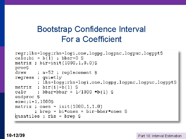
Bootstrap Confidence Interval For a Coefficient 10 -12/39 Part 10: Interval Estimation

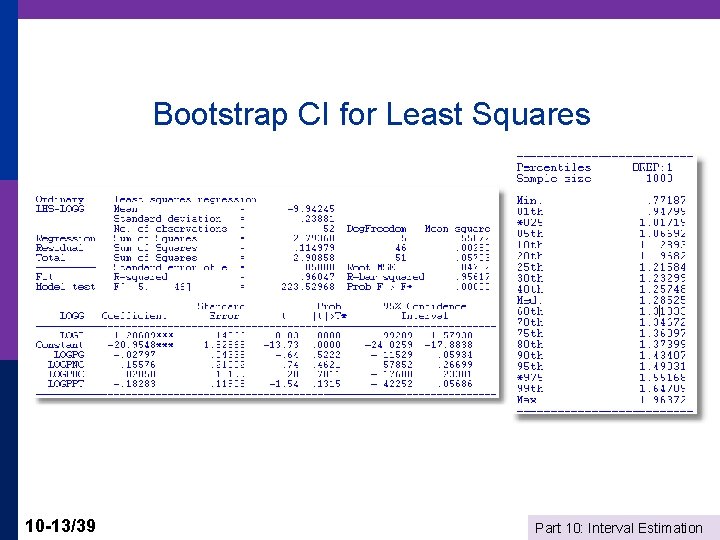
Bootstrap CI for Least Squares 10 -13/39 Part 10: Interval Estimation

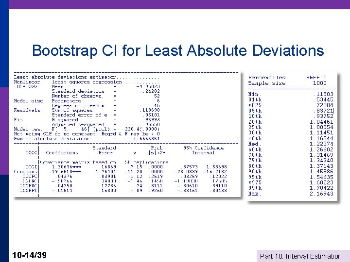
Bootstrap CI for Least Absolute Deviations 10 -14/39 Part 10: Interval Estimation

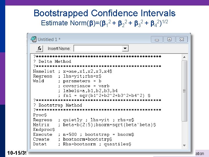
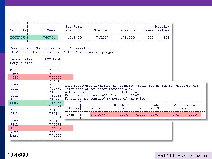
Bootstrapped Confidence Intervals Estimate Norm( )=( 12 + 22 + 32 + 42)1/2 10 -15/39 Part 10: Interval Estimation

10 -16/39 Part 10: Interval Estimation

10 -17/39 Part 10: Interval Estimation

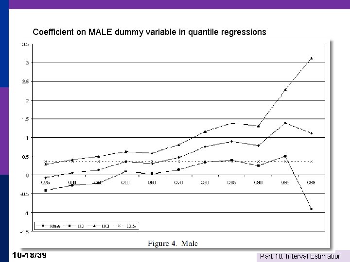
Coefficient on MALE dummy variable in quantile regressions 10 -18/39 Part 10: Interval Estimation

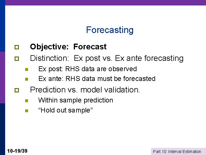
Forecasting Objective: Forecast Distinction: Ex post vs. Ex ante forecasting p p n n Ex post: RHS data are observed Ex ante: RHS data must be forecasted Prediction vs. model validation. p n n 10 -19/39 Within sample prediction “Hold out sample” Part 10: Interval Estimation

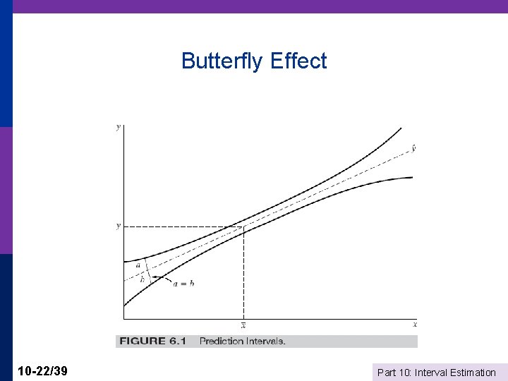
Prediction Intervals Given x 0 predict y 0. Two cases: Estimate E[y|x 0] = x 0; Predict y 0 = x 0 + 0 Obvious predictor, b’x 0 + estimate of 0. Forecast 0 as 0, but allow for variance. Alternative: When we predict y 0 with b x 0, what is the 'forecast error? ' Est. y 0 - y 0 = b x 0 - 0, so the variance of the forecast error is x 0 Var[b - ]x 0 + 2 How do we estimate this? Form a confidence interval. Two cases: If x 0 is a vector of constants, the variance is just x 0 Var[b] x 0. Form confidence interval as usual. If x 0 had to be estimated, then we use a random variable. What is the variance of the product? (Ouch!) One possibility: Use bootstrapping. 10 -20/39 Part 10: Interval Estimation

Forecast Variance of the forecast error is 2 + x 0’ Var[b]x 0 = 2 + 2[x 0’(X’X)-1 x 0] If the model contains a constant term, this is In terms squares and cross products of deviations from means. Interpretation: Forecast variance is smallest in the middle of our “experience” and increases as we move outside it. 10 -21/39 Part 10: Interval Estimation

Butterfly Effect 10 -22/39 Part 10: Interval Estimation

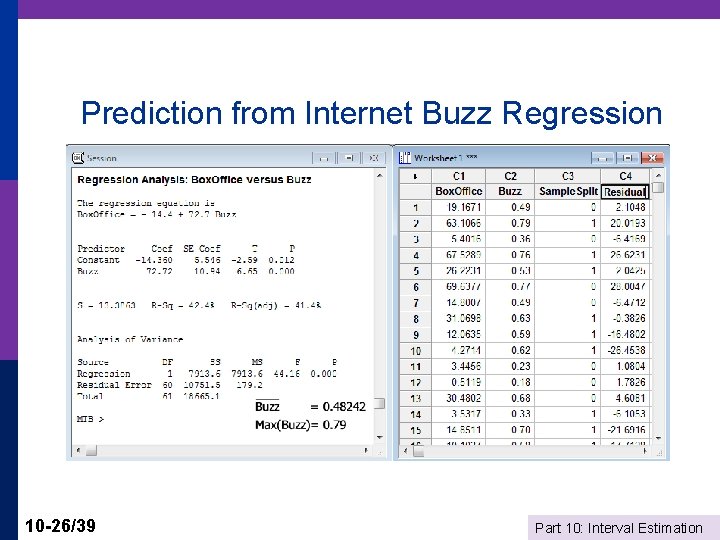
Internet Buzz Data 10 -23/39 Part 10: Interval Estimation

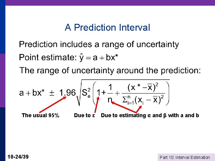
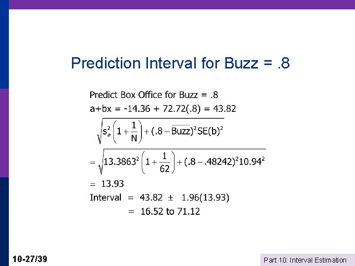
A Prediction Interval The usual 95% 10 -24/39 Due to ε Due to estimating α and β with a and b Part 10: Interval Estimation

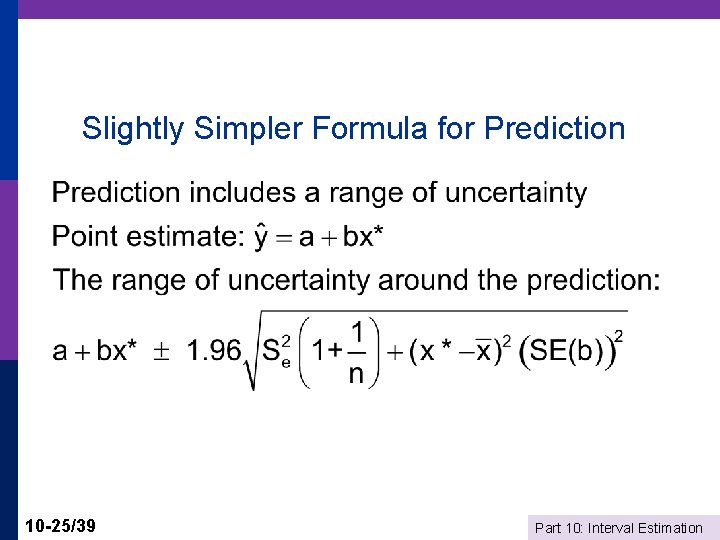
Slightly Simpler Formula for Prediction 10 -25/39 Part 10: Interval Estimation

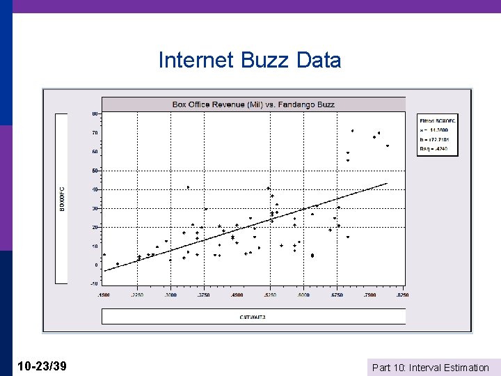
Prediction from Internet Buzz Regression 10 -26/39 Part 10: Interval Estimation

Prediction Interval for Buzz =. 8 10 -27/39 Part 10: Interval Estimation

Semi- and Nonparametric Estimation 10 -/39 Part 10: Interval Estimation

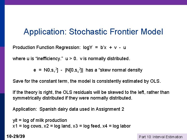
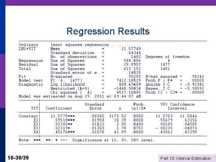
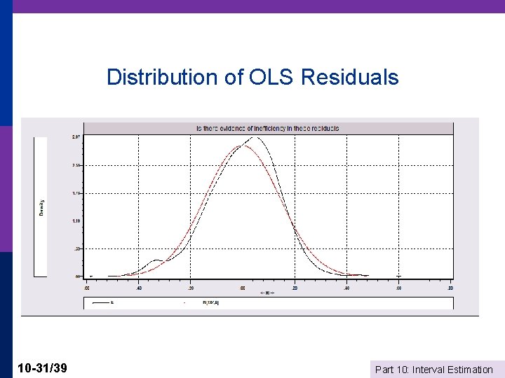
Application: Stochastic Frontier Model Production Function Regression: log. Y = b’x + v - u where u is “inefficiency. ” u > 0. v is normally distributed. e = N 0, sv 2] - |N[0, su 2]| has a “skew normal density Save for the constant term, the model is consistently estimated by OLS. If theory is right, the OLS residuals will be skewed to the left, rather than symmetrically distributed if they were normally distributed. Application: Spanish dairy data used in Assignment 2 yit = log of milk production x 1 = log cows, x 2 = log land, x 3 = log feed, x 4 = log labor 10 -29/39 Part 10: Interval Estimation

Regression Results 10 -30/39 Part 10: Interval Estimation

Distribution of OLS Residuals 10 -31/39 Part 10: Interval Estimation

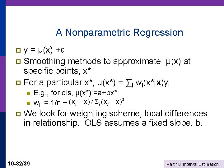
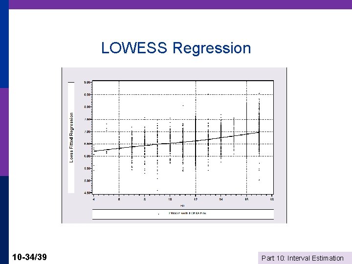
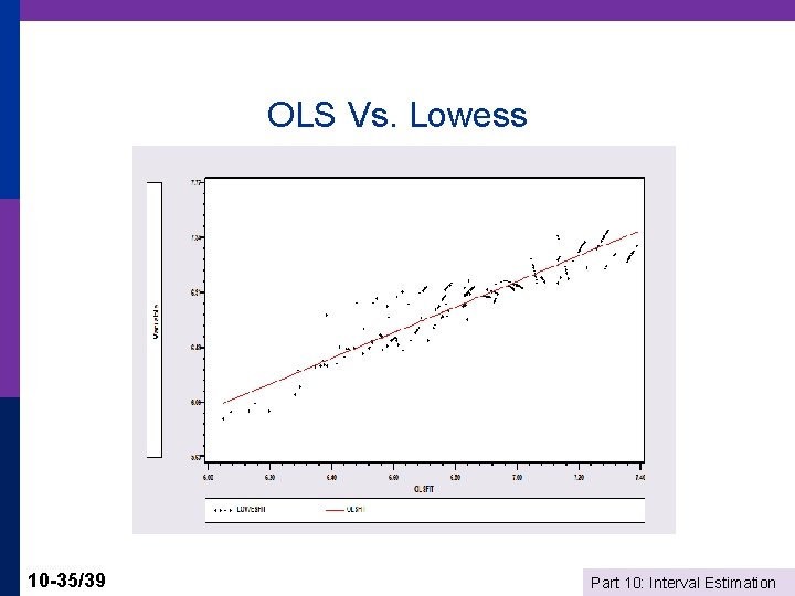
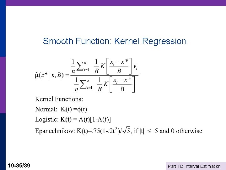
A Nonparametric Regression y = µ(x) +ε p Smoothing methods to approximate µ(x) at specific points, x* p For a particular x*, µ(x*) = ∑i wi(x*|x)yi p n n p E. g. , for ols, µ(x*) =a+bx* wi = 1/n + We look for weighting scheme, local differences in relationship. OLS assumes a fixed slope, b. 10 -32/39 Part 10: Interval Estimation

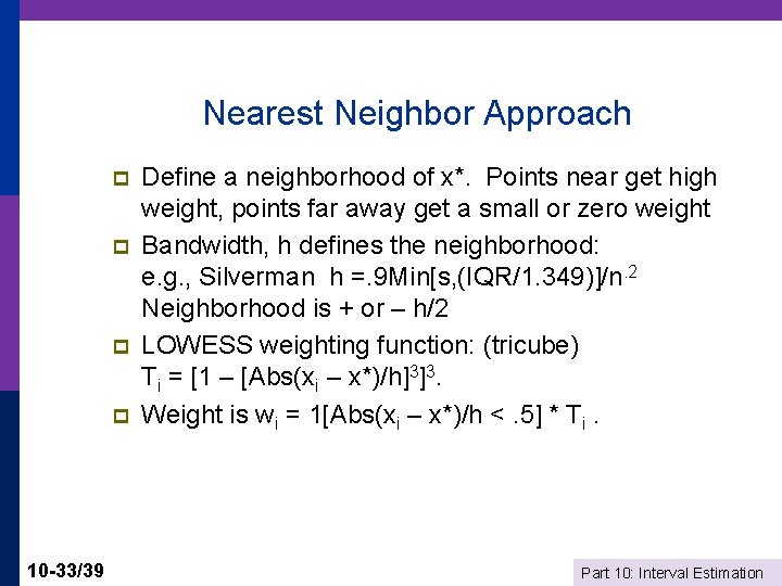
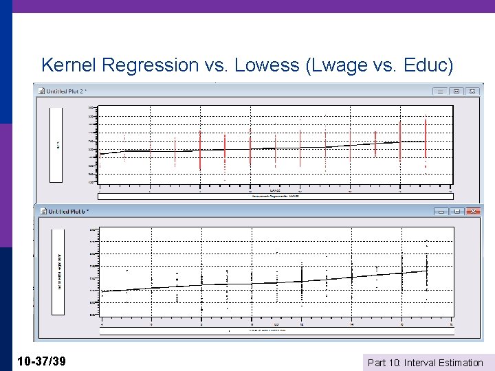
Nearest Neighbor Approach p p 10 -33/39 Define a neighborhood of x*. Points near get high weight, points far away get a small or zero weight Bandwidth, h defines the neighborhood: e. g. , Silverman h =. 9 Min[s, (IQR/1. 349)]/n. 2 Neighborhood is + or – h/2 LOWESS weighting function: (tricube) Ti = [1 – [Abs(xi – x*)/h]3]3. Weight is wi = 1[Abs(xi – x*)/h <. 5] * Ti. Part 10: Interval Estimation

LOWESS Regression 10 -34/39 Part 10: Interval Estimation

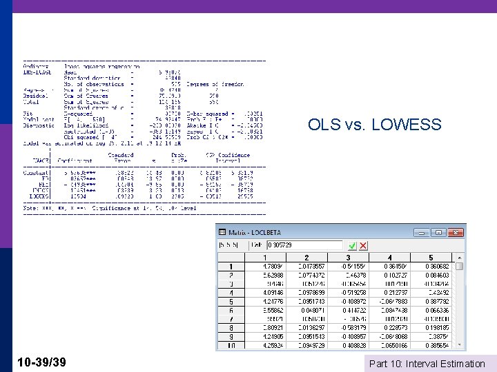
OLS Vs. Lowess 10 -35/39 Part 10: Interval Estimation

Smooth Function: Kernel Regression 10 -36/39 Part 10: Interval Estimation

Kernel Regression vs. Lowess (Lwage vs. Educ) 10 -37/39 Part 10: Interval Estimation

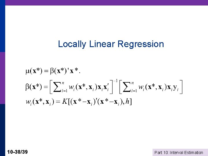
Locally Linear Regression 10 -38/39 Part 10: Interval Estimation

OLS vs. LOWESS 10 -39/39 Part 10: Interval Estimation