Differential and Integral Calculus Unit 2 Differential and

Differential and Integral Calculus Unit 2

Differential and Integral Calculus n Calculus is the study of “Rates of Change”. ¨ In a linear function, the slope (m) expresses the rate of change of the function. ¨ Example, assume the following linear function: y = mx + 20 n Positive slope: increase in x increase in y n Negative slope: increase in x decrease in y

Differential and Integral Calculus n Calculus is the study of “Rates of Change”. ¨ In a linear function, the slope (m) expresses the rate of change of the function. ¨ Example, assume the following linear function: y = mx + 20 n y = 5 x + 20; every 1 -unit increase in x causes a 5 unit increase in y = -5 x + 20; every 1 -unit increase in x causes a 5 unit decrease in y

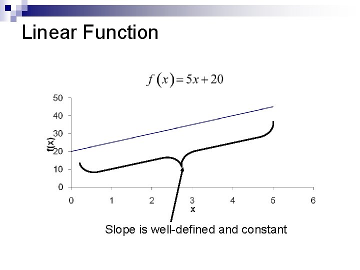
Linear Function Slope is well-defined and constant

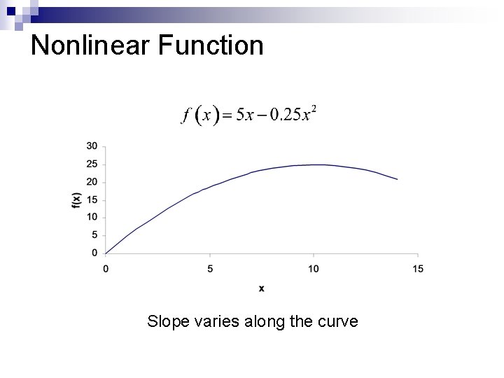
Nonlinear Function Slope varies along the curve

Differential and Integral Calculus n Calculus is the study of “Rates of Change”. ¨ Calculus is used to determine the slope of a curve at a specific point on the curve. ¨ Business applications: marginal revenue, marginal cost, profit maximization, diminishing marginal returns, efficiency, etc.

Differential and Integral Calculus n n n Differential calculus determines the rate of change of a quantity. (Chapters 11 -14) Multivariate calculus works with more than one variable (Chapter 17) Integral calculus determines the quantity where the rate of change is known. (Chapter 15)

Differential Calculus Chapter 11

The Derivative n n n 11. 1 Limits 11. 3 Rates of Change 11. 4 Definition of the Derivative

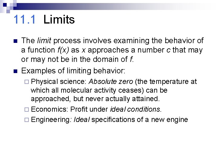
11. 1 Limits n n The limit process involves examining the behavior of a function f(x) as x approaches a number c that may or may not be in the domain of f. Examples of limiting behavior: ¨ Physical science: Absolute zero (the temperature at which all molecular activity ceases) can be approached, but never actually attained. ¨ Economics: Profit under ideal conditions. ¨ Engineering: Ideal specifications of a new engine

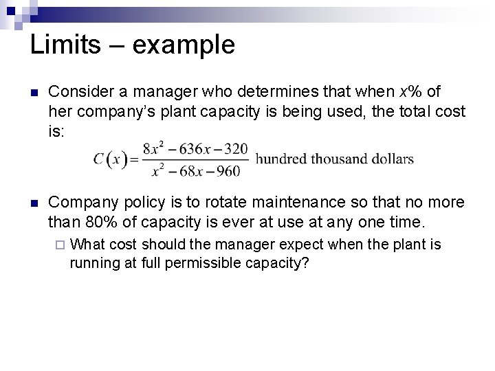
Limits – example n Consider a manager who determines that when x% of her company’s plant capacity is being used, the total cost is: n Company policy is to rotate maintenance so that no more than 80% of capacity is ever at use at any one time. ¨ What cost should the manager expect when the plant is running at full permissible capacity?

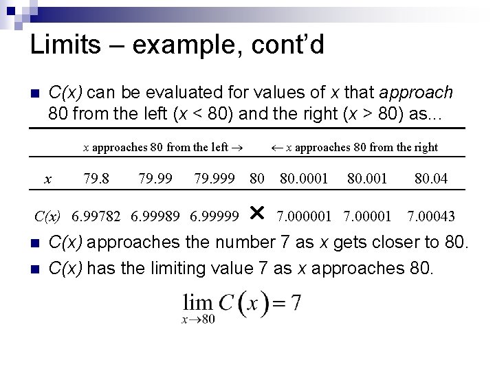
Limits – example, cont’d n C(x) can be evaluated for values of x that approach 80 from the left (x < 80) and the right (x > 80) as. . . x approaches 80 from the left x 79. 8 79. 999 80 80. 0001 C(x) 6. 99782 6. 99989 6. 99999 n n x approaches 80 from the right 80. 001 80. 04 7. 000001 7. 00043 C(x) approaches the number 7 as x gets closer to 80. C(x) has the limiting value 7 as x approaches 80.

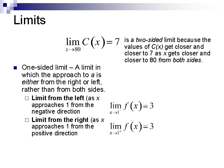
Limits n n One-sided limit – A limit in which the approach to a is either from the right or left, rather than from both sides. Limit from the left (as x approaches 1 from the negative direction ¨ Limit from the right (as x approaches 1 from the positive direction ¨ is a two-sided limit because the values of C(x) get closer and closer to 7 as x gets closer and closer to 80 from both sides.

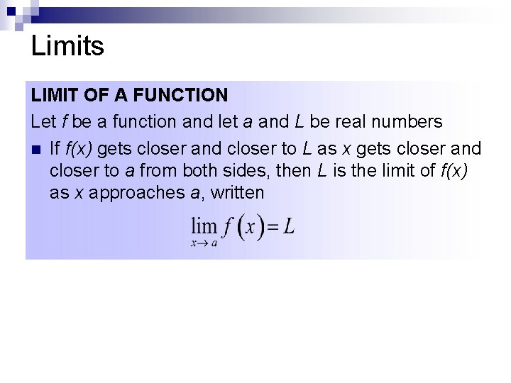
Limits LIMIT OF A FUNCTION Let f be a function and let a and L be real numbers n If f(x) gets closer and closer to L as x gets closer and closer to a from both sides, then L is the limit of f(x) as x approaches a, written

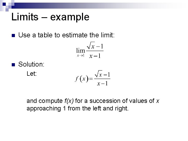
Limits – example n Use a table to estimate the limit: n Solution: ¨ Let: ¨ and compute f(x) for a succession of values of x approaching 1 from the left and right.

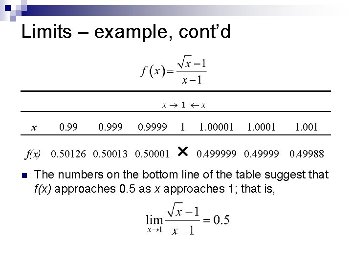
Limits – example, cont’d x 1 x x 0. 9999 1 1. 00001 f(x) 0. 50126 0. 50013 0. 50001 0. 499999 0. 49988 n 0. 999 1. 0001 1. 001 The numbers on the bottom line of the table suggest that f(x) approaches 0. 5 as x approaches 1; that is,

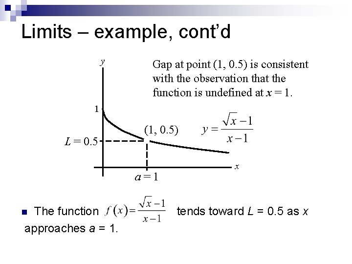
Limits – example, cont’d y Gap at point (1, 0. 5) is consistent with the observation that the function is undefined at x = 1. 1 L = 0. 5 (1, 0. 5) a=1 The function approaches a = 1. n x tends toward L = 0. 5 as x

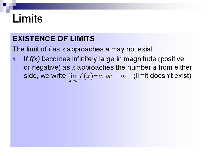
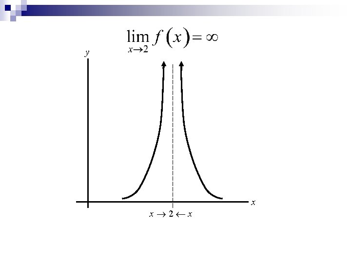
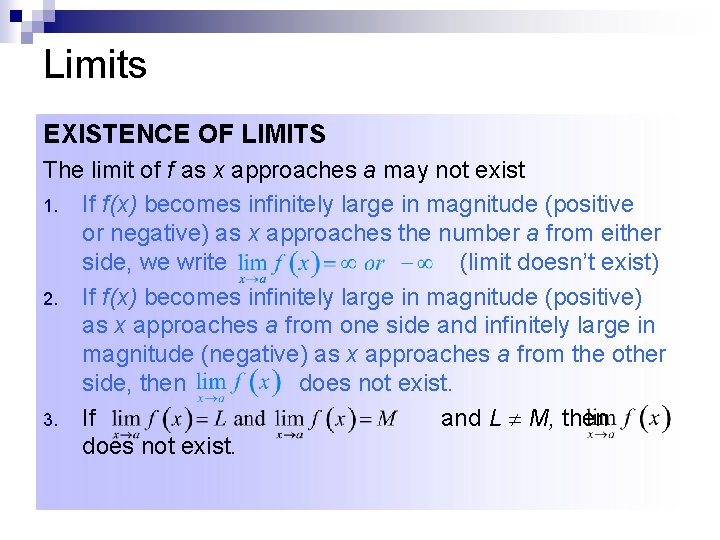
Limits EXISTENCE OF LIMITS The limit of f as x approaches a may not exist 1. If f(x) becomes infinitely large in magnitude (positive or negative) as x approaches the number a from either side, we write (limit doesn’t exist)

y x 2 x x

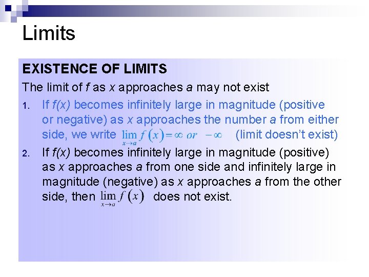
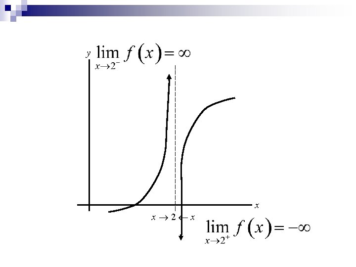
Limits EXISTENCE OF LIMITS The limit of f as x approaches a may not exist 1. If f(x) becomes infinitely large in magnitude (positive or negative) as x approaches the number a from either side, we write (limit doesn’t exist) 2. If f(x) becomes infinitely large in magnitude (positive) as x approaches a from one side and infinitely large in magnitude (negative) as x approaches a from the other side, then does not exist.

y x 2 x x

Limits EXISTENCE OF LIMITS The limit of f as x approaches a may not exist 1. If f(x) becomes infinitely large in magnitude (positive or negative) as x approaches the number a from either side, we write (limit doesn’t exist) 2. If f(x) becomes infinitely large in magnitude (positive) as x approaches a from one side and infinitely large in magnitude (negative) as x approaches a from the other side, then does not exist. 3. If and L M, then does not exist.

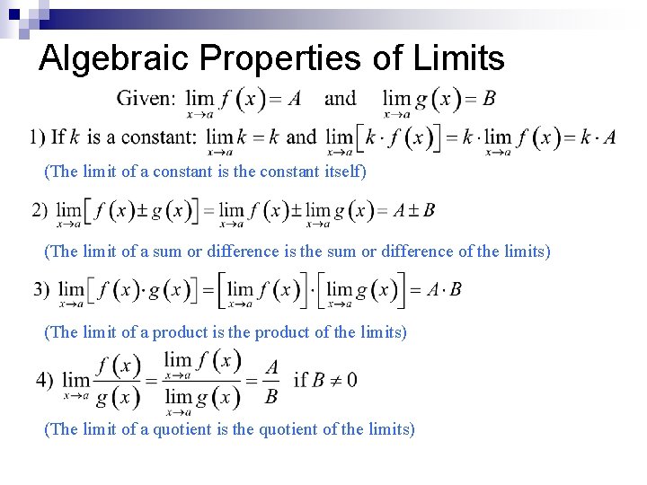
Algebraic Properties of Limits (The limit of a constant is the constant itself) (The limit of a sum or difference is the sum or difference of the limits) (The limit of a product is the product of the limits) (The limit of a quotient is the quotient of the limits)

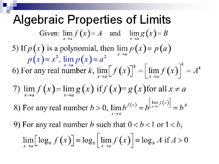
Algebraic Properties of Limits

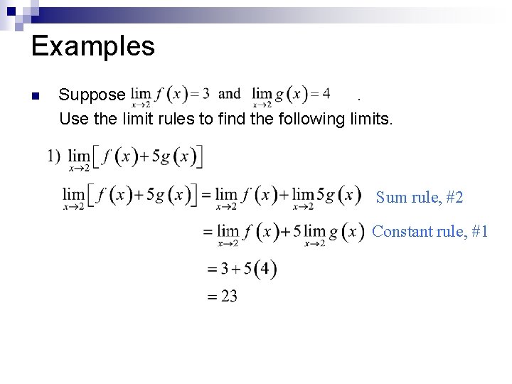
Examples n Suppose. Use the limit rules to find the following limits. Sum rule, #2 Constant rule, #1

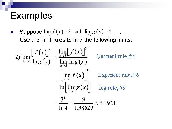
Examples n Suppose. Use the limit rules to find the following limits. Quotient rule, #4 Exponent rule, #6 log rule, #9

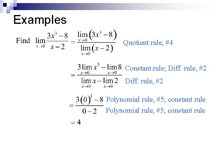
Examples Quotient rule, #4 Constant rule; Diff. rule, #2 Polynomial rule, #5; constant rule

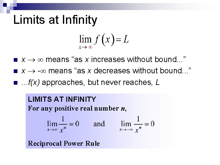
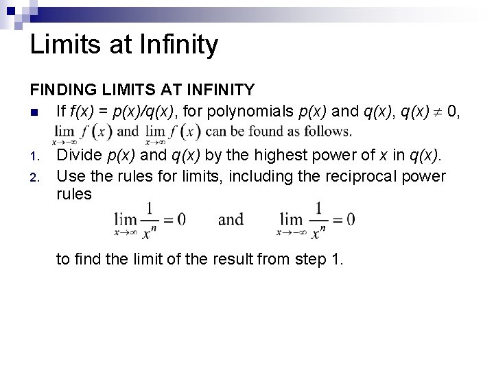
Limits at Infinity n n n x means “as x increases without bound. . . ” x - means “as x decreases without bound. . . ”. . . f(x) approaches, but never reaches, L LIMITS AT INFINITY For any positive real number n, Reciprocal Power Rule

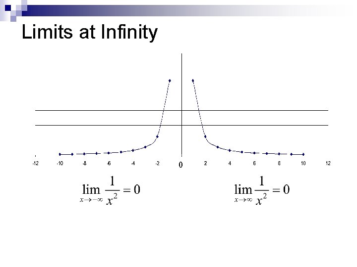
Limits at Infinity 0

Limits at Infinity FINDING LIMITS AT INFINITY n If f(x) = p(x)/q(x), for polynomials p(x) and q(x), q(x) 0, 1. 2. Divide p(x) and q(x) by the highest power of x in q(x). Use the rules for limits, including the reciprocal power rules to find the limit of the result from step 1.

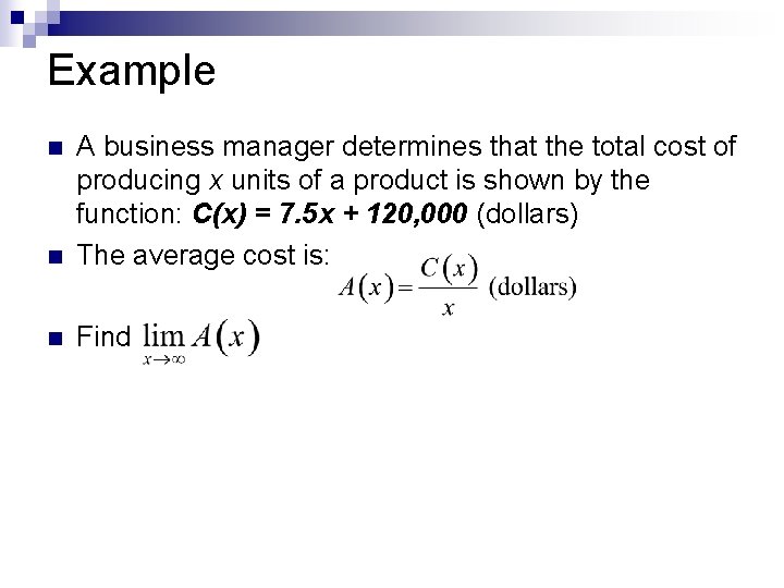
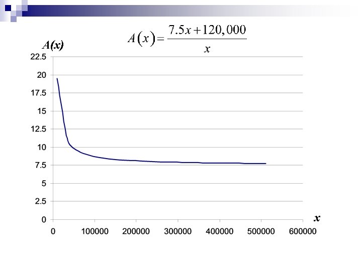
Example n A business manager determines that the total cost of producing x units of a product is shown by the function: C(x) = 7. 5 x + 120, 000 (dollars) The average cost is: n Find n

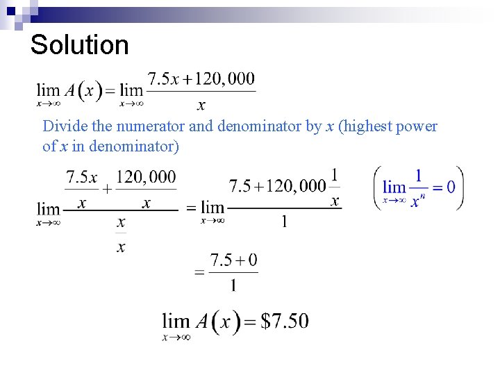
Solution Divide the numerator and denominator by x (highest power of x in denominator)

A(x) x

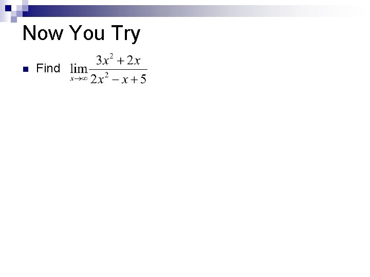
Now You Try n Find

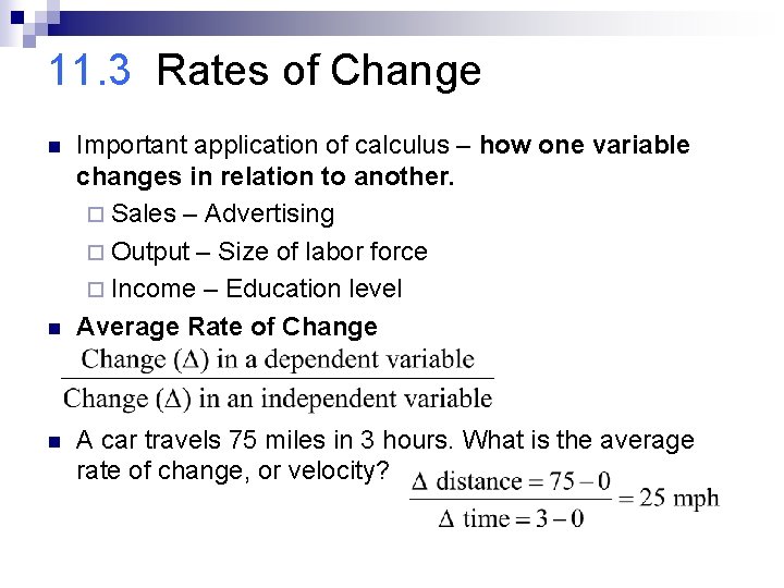
11. 3 Rates of Change n n n Important application of calculus – how one variable changes in relation to another. ¨ Sales – Advertising ¨ Output – Size of labor force ¨ Income – Education level Average Rate of Change A car travels 75 miles in 3 hours. What is the average rate of change, or velocity?

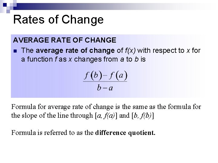
Rates of Change AVERAGE RATE OF CHANGE n The average rate of change of f(x) with respect to x for a function f as x changes from a to b is Formula for average rate of change is the same as the formula for the slope of the line through [a, f(a)] and [b, f(b)] Formula is referred to as the difference quotient.

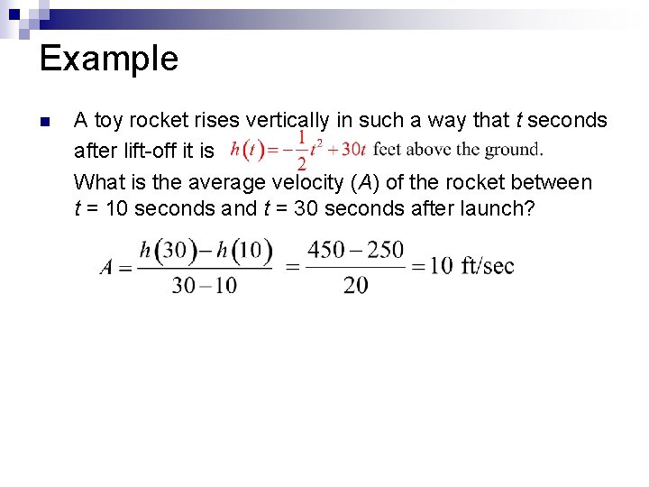
Example n n n A toy rocket rises vertically in such a way that t seconds after lift-off it is What is the average velocity (A) of the rocket between t = 10 seconds and t = 30 seconds after launch?

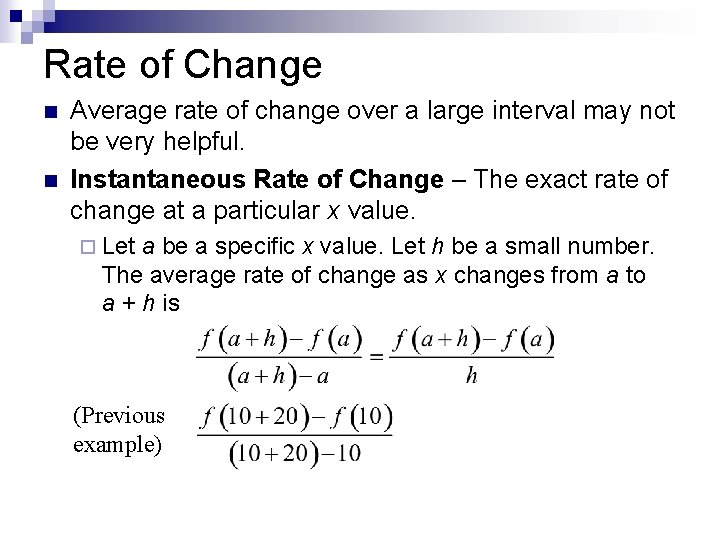
Rate of Change n n Average rate of change over a large interval may not be very helpful. Instantaneous Rate of Change – The exact rate of change at a particular x value. ¨ Let a be a specific x value. Let h be a small number. The average rate of change as x changes from a to a + h is (Previous example)

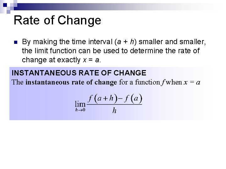
Rate of Change n By making the time interval (a + h) smaller and smaller, the limit function can be used to determine the rate of change at exactly x = a. INSTANTANEOUS RATE OF CHANGE The instantaneous rate of change for a function f when x = a

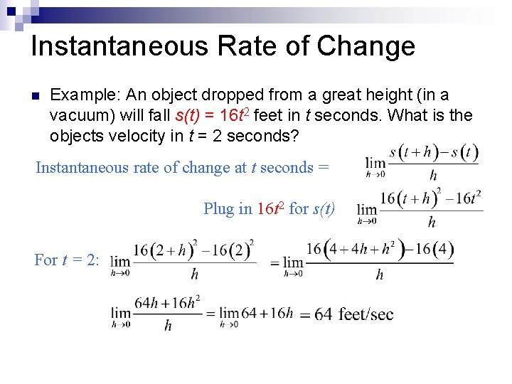
Instantaneous Rate of Change n Example: An object dropped from a great height (in a vacuum) will fall s(t) = 16 t 2 feet in t seconds. What is the objects velocity in t = 2 seconds? Instantaneous rate of change at t seconds = Plug in 16 t 2 for s(t) For t = 2:

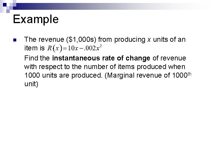
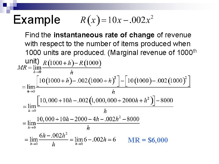
Example The revenue ($1, 000 s) from producing x units of an item is b. Find the instantaneous rate of change of revenue with respect to the number of items produced when 1000 units are produced. (Marginal revenue of 1000 th unit) n

Example b. Find the instantaneous rate of change of revenue with respect to the number of items produced when 1000 units are produced. (Marginal revenue of 1000 th unit) MR = $6, 000

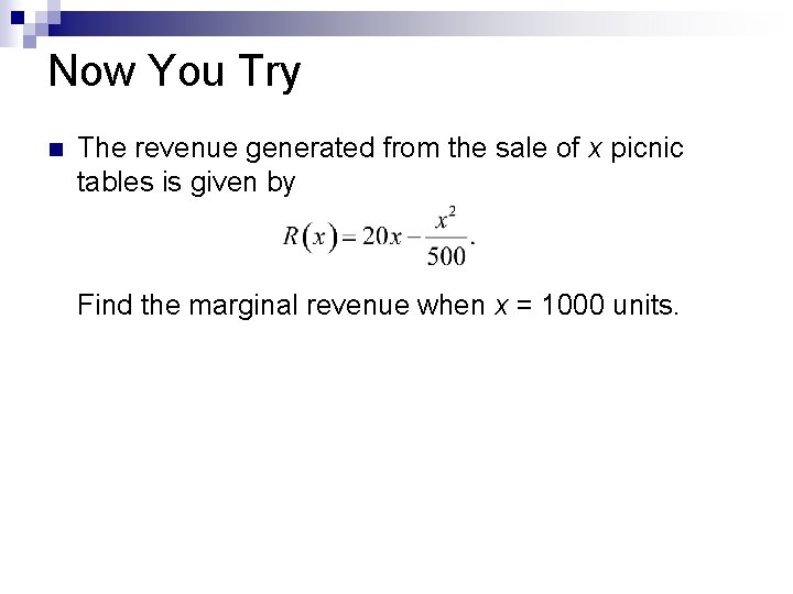
Now You Try n The revenue generated from the sale of x picnic tables is given by n Find the marginal revenue when x = 1000 units.

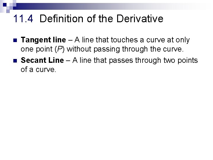
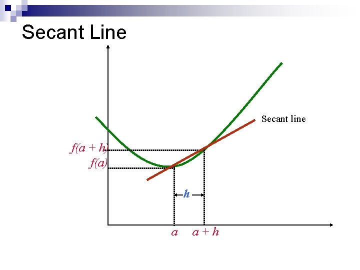
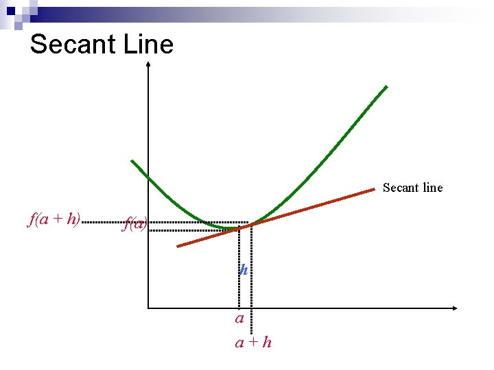
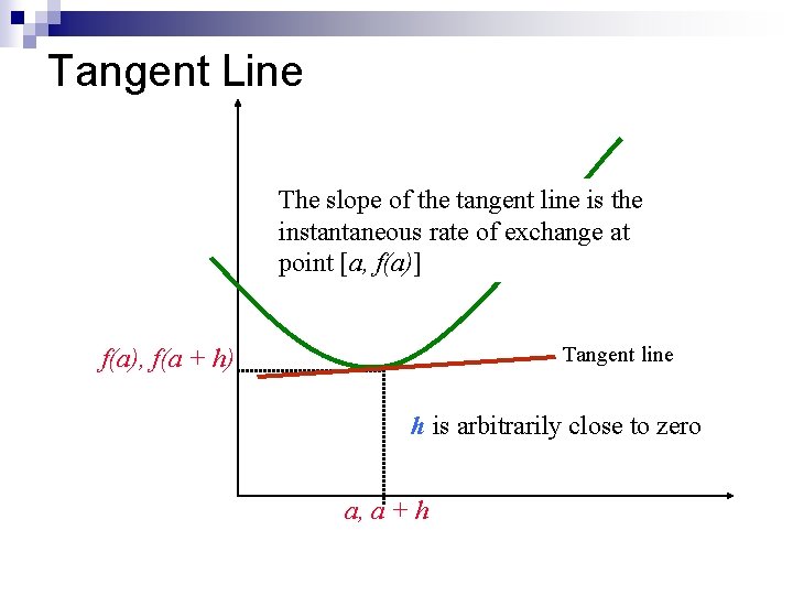
11. 4 Definition of the Derivative n n Tangent line – A line that touches a curve at only one point (P) without passing through the curve. Secant Line – A line that passes through two points of a curve.

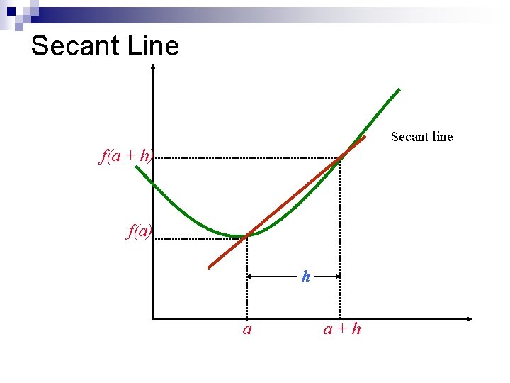
Secant Line Secant line f(a + h) f(a) h a a+h

Secant Line Secant line f(a + h) f(a) h a a+h

Secant Line Secant line f(a + h) f(a) h a a+h

Tangent Line The slope of the tangent line is the instantaneous rate of exchange at point [a, f(a)] Tangent line f(a), f(a + h) h is arbitrarily close to zero a, a + h

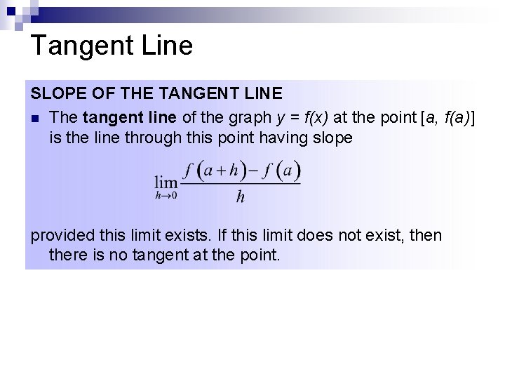
Tangent Line SLOPE OF THE TANGENT LINE n The tangent line of the graph y = f(x) at the point [a, f(a)] is the line through this point having slope provided this limit exists. If this limit does not exist, then there is no tangent at the point.

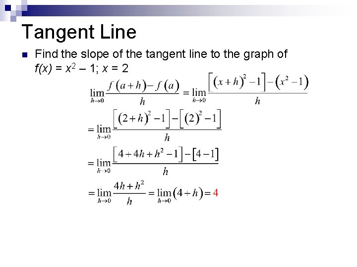
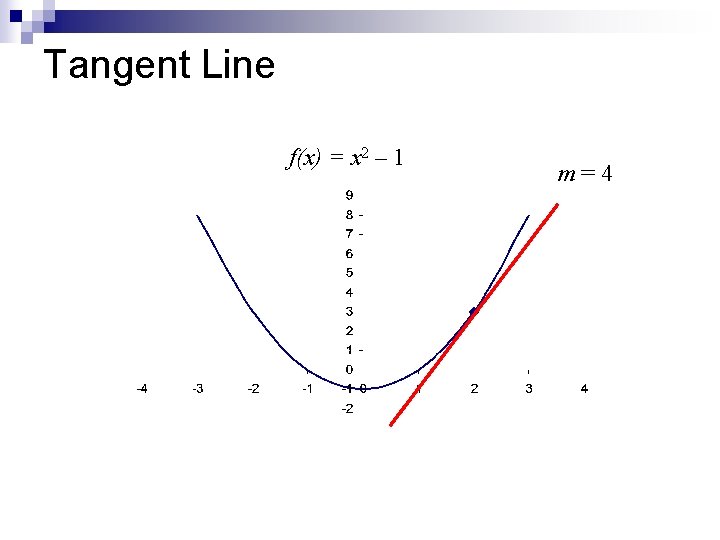
Tangent Line n Find the slope of the tangent line to the graph of f(x) = x 2 – 1; x = 2

Tangent Line f(x) = x 2 – 1 m=4

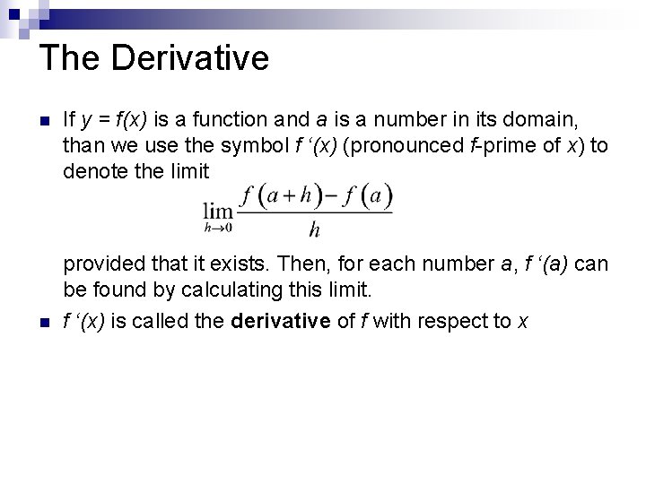
The Derivative n If y = f(x) is a function and a is a number in its domain, than we use the symbol f ‘(x) (pronounced f-prime of x) to denote the limit n provided that it exists. Then, for each number a, f ‘(a) can be found by calculating this limit. f ‘(x) is called the derivative of f with respect to x n

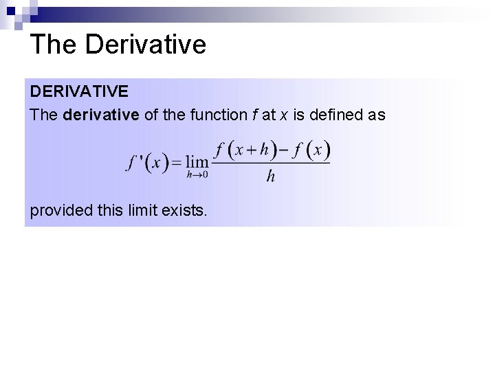
The Derivative DERIVATIVE The derivative of the function f at x is defined as provided this limit exists.

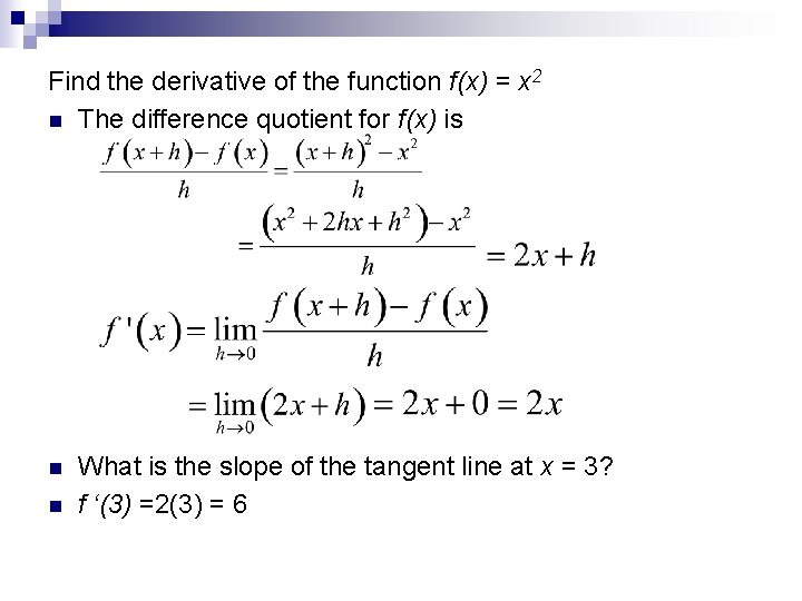
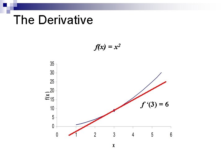
Find the derivative of the function f(x) = x 2 n The difference quotient for f(x) is n n What is the slope of the tangent line at x = 3? f ‘(3) =2(3) = 6

The Derivative f(x) = x 2 f ‘(3) = 6

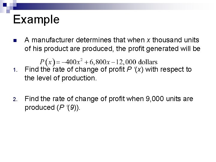
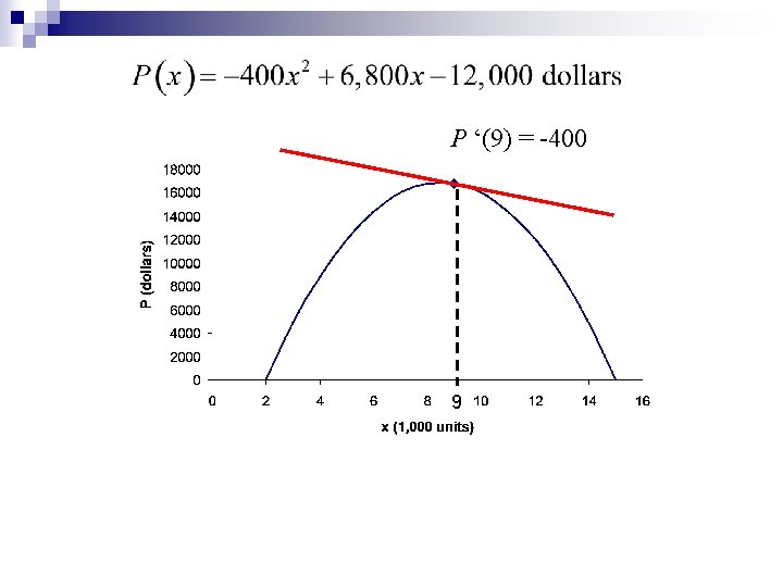
Example n A manufacturer determines that when x thousand units of his product are produced, the profit generated will be 1. Find the rate of change of profit P ‘(x) with respect to the level of production. 2. Find the rate of change of profit when 9, 000 units are produced (P ‘(9)).

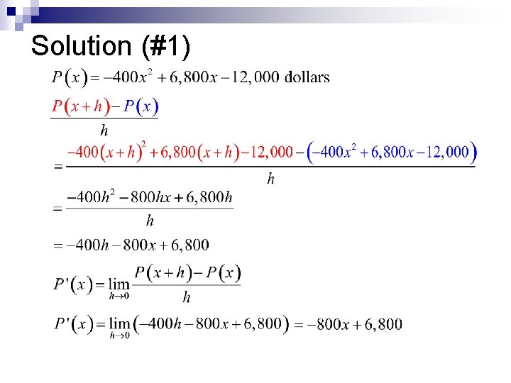
Solution (#1)

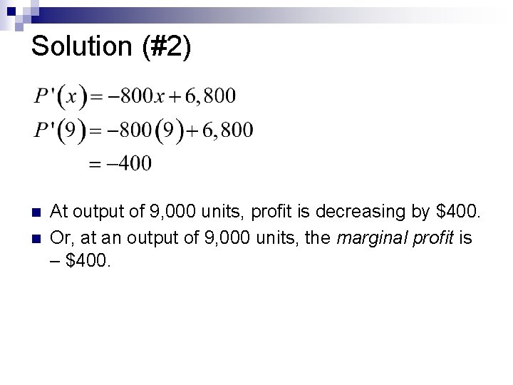
Solution (#2) n n At output of 9, 000 units, profit is decreasing by $400. Or, at an output of 9, 000 units, the marginal profit is – $400.

P ‘(9) = -400 9

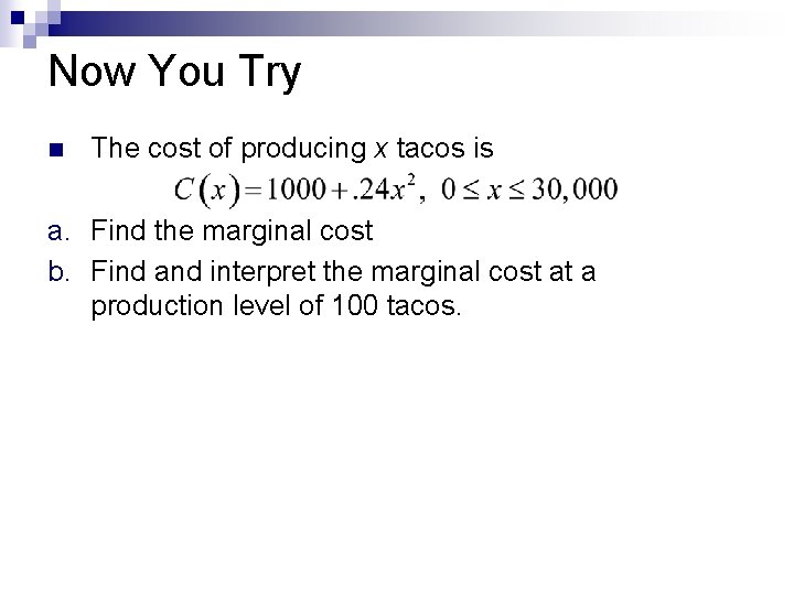
Now You Try n The cost of producing x tacos is a. Find the marginal cost b. Find and interpret the marginal cost at a production level of 100 tacos.

Chapter 11 End