DIFFERENTIAL CALCULUS Outcomes for this session Introduction Calculus

DIFFERENTIAL CALCULUS

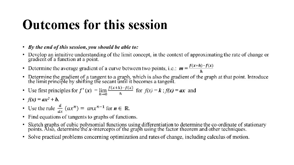
Outcomes for this session •

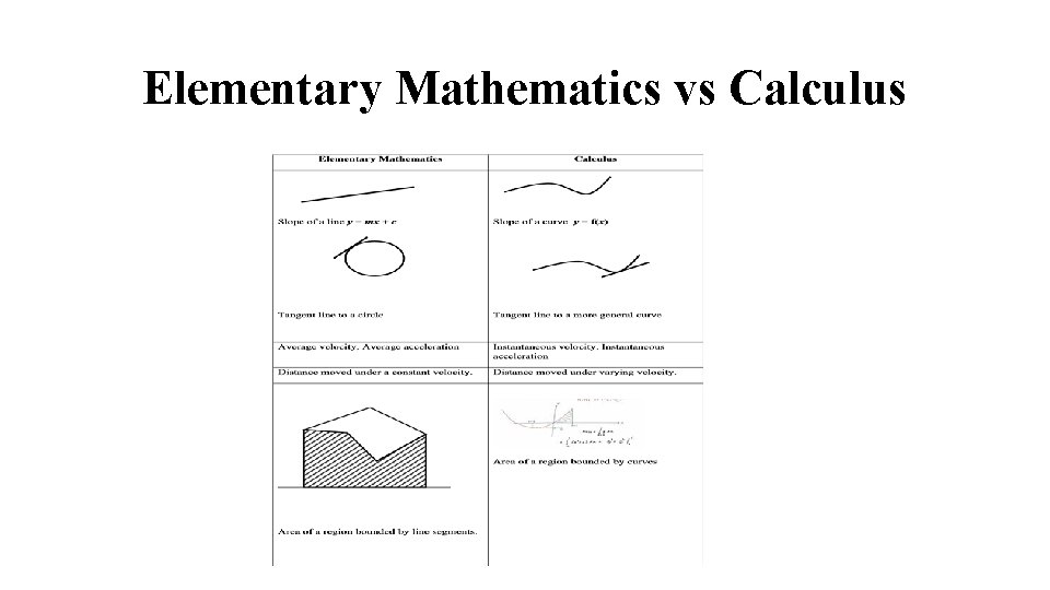
Introduction • Calculus is a branch of mathematics involving or leading to calculations dealing with continuously varying functions. • To a Roman in the days of the empire a “calculus” was a pebble used in counting and gambling. • Centuries later “calculare” came to mean “to compute”, “to reckon”, “to figure out”. To the mathematician, physical scientist, and social scientist of today, calculus is elementary mathematics (algebra, geometry, trigonometry) enhanced by the limit process. • Calculus takes ideas from elementary mathematics and extends them to a more general situation. • The table below contains some examples. On the left-hand side, you will find an idea from elementary mathematics; on the right, this same idea as extended by calculus

Elementary Mathematics vs Calculus

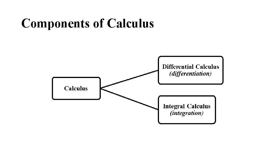
Components of Calculus

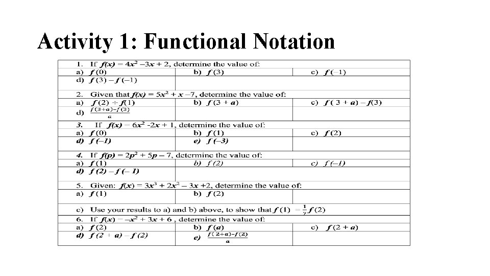
Activity 1: Functional Notation

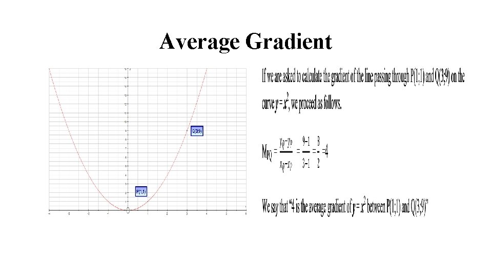
Average Gradient

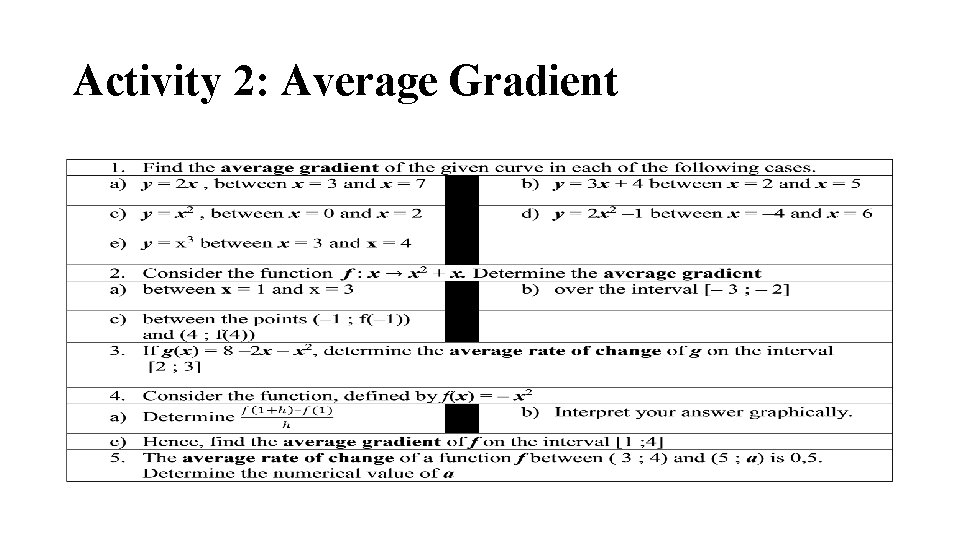
Activity 2: Average Gradient

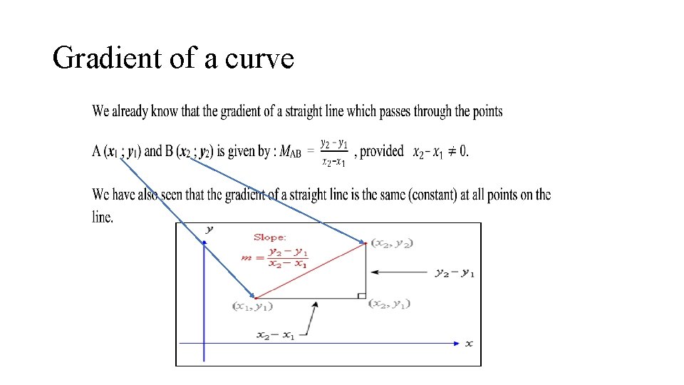
Gradient of a curve

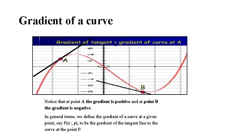
Gradient of a curve Notice that at point A the gradient is positive and at point B the gradient is negative. In general terms, we define the gradient of a curve at a given point, say P(x ; y), to be the gradient of the tangent line to the curve at the point P.

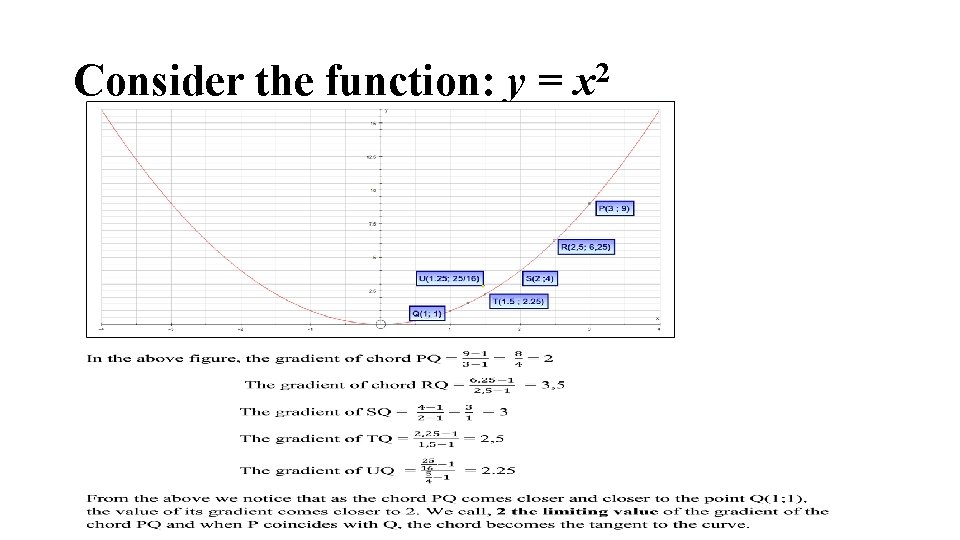
Consider the function: y = x 2

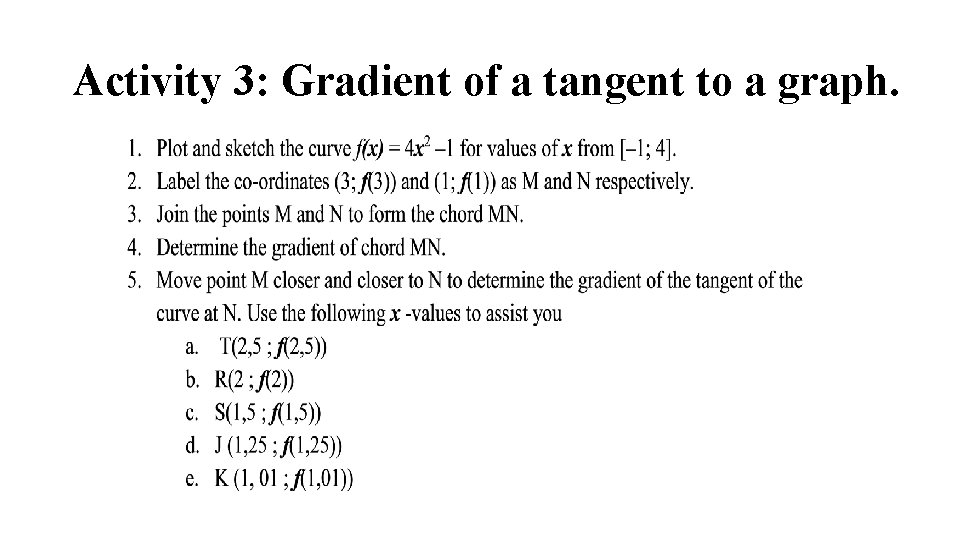
Activity 3: Gradient of a tangent to a graph.

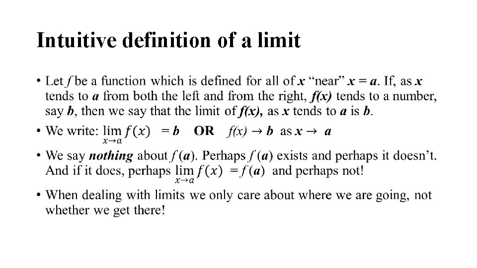
Intuitive definition of a limit •

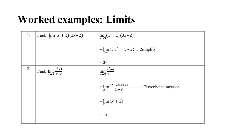
Worked examples: Limits

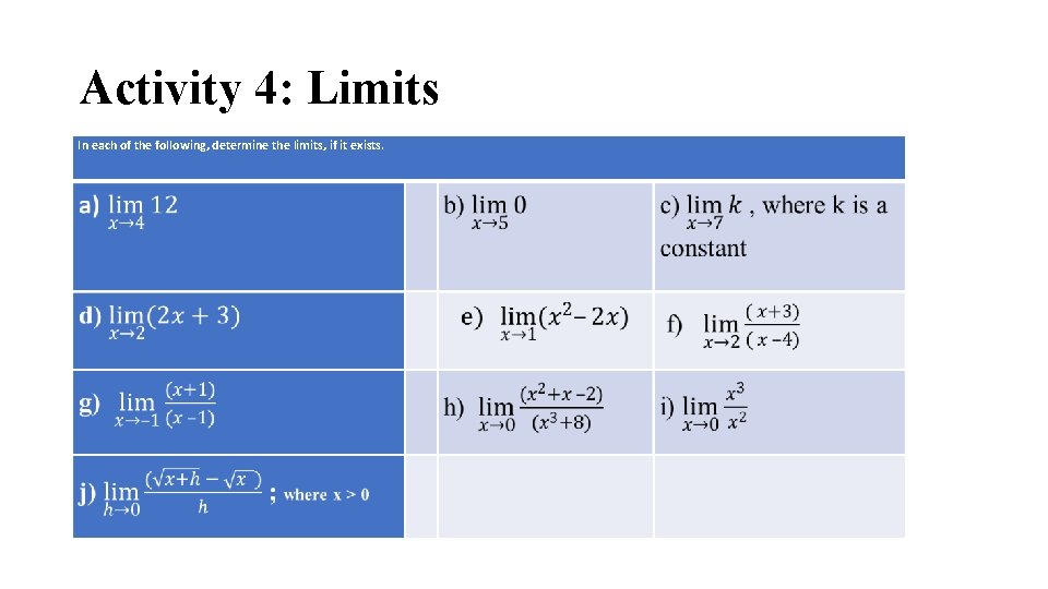
Activity 4: Limits In each of the following, determine the limits, if it exists.

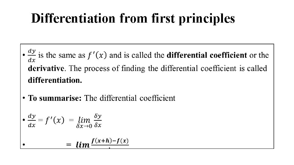
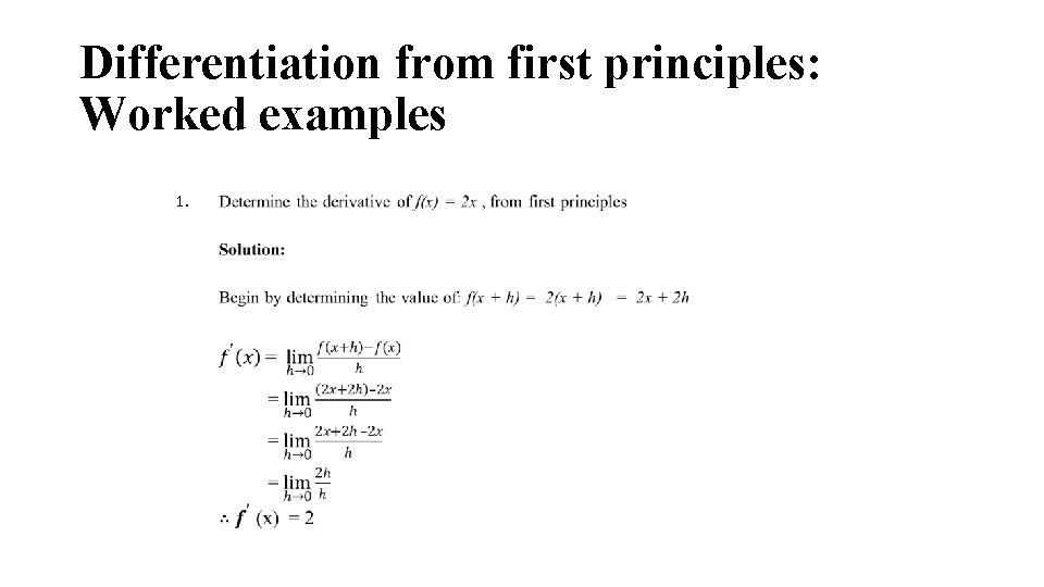
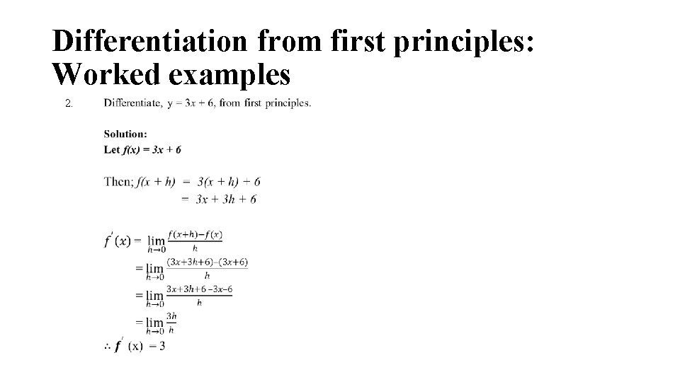
Differentiation from first principles •

Differentiation from first principles: Worked examples 1.

Differentiation from first principles: Worked examples 2.

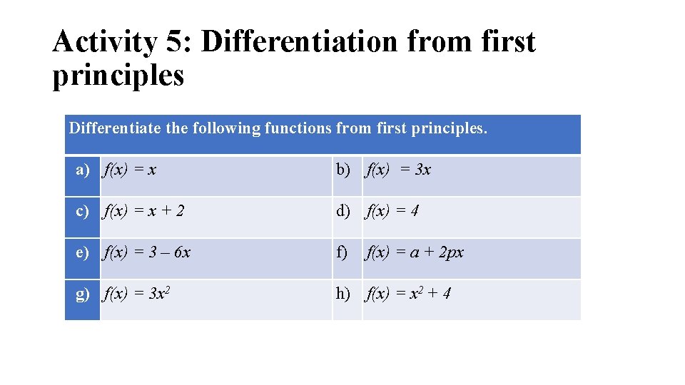
Activity 5: Differentiation from first principles Differentiate the following functions from first principles. a) f(x) = x b) f(x) = 3 x c) f(x) = x + 2 d) f(x) = 4 e) f(x) = 3 – 6 x f) g) f(x) = 3 x 2 h) f(x) = x 2 + 4 f(x) = a + 2 px

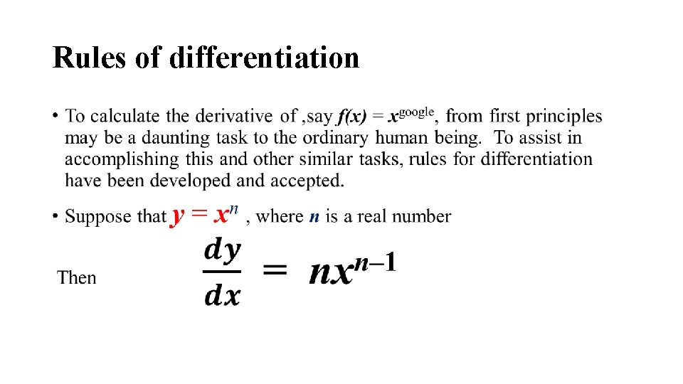
Rules of differentiation •

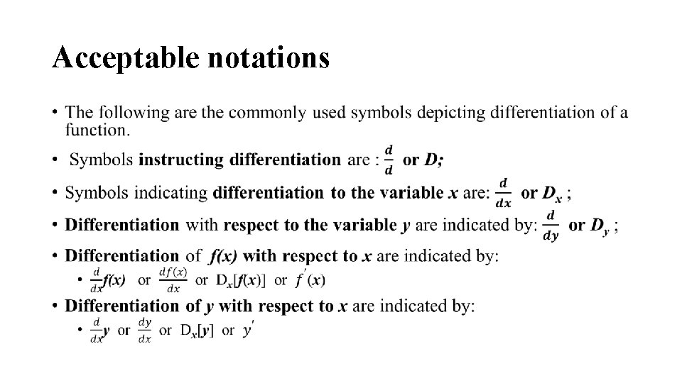
Acceptable notations •

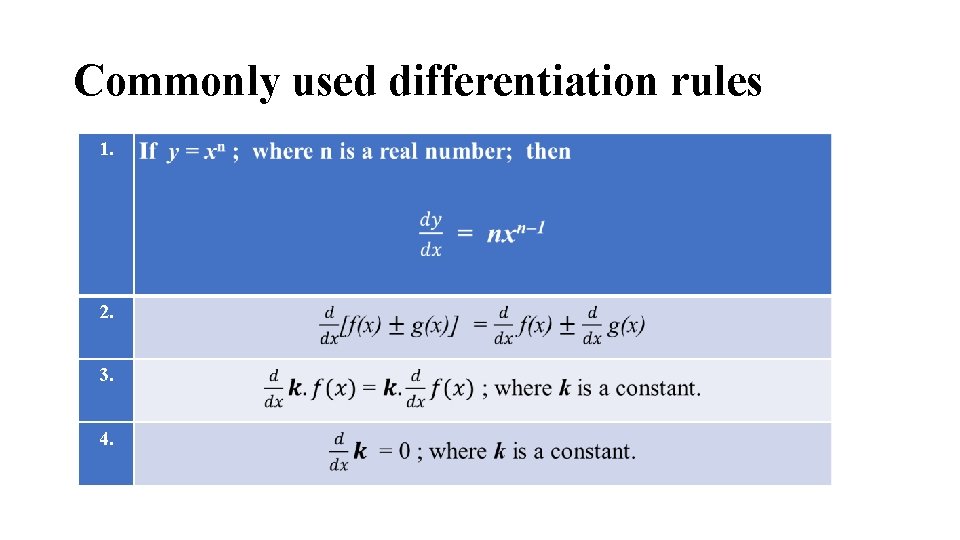
Commonly used differentiation rules 1. 2. 3. 4.

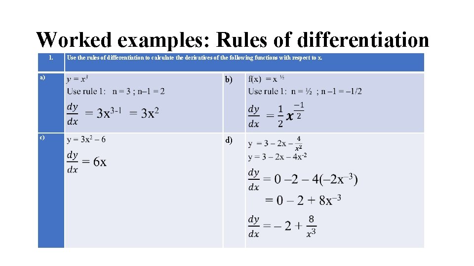
Worked examples: Rules of differentiation 1. Use the rules of differentiation to calculate the derivatives of the following functions with respect to x. a) b) c) d)

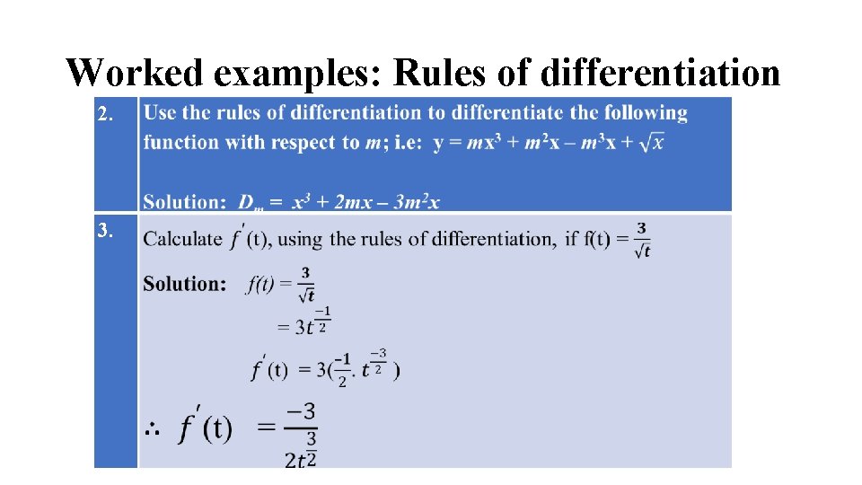
Worked examples: Rules of differentiation 2. 3.

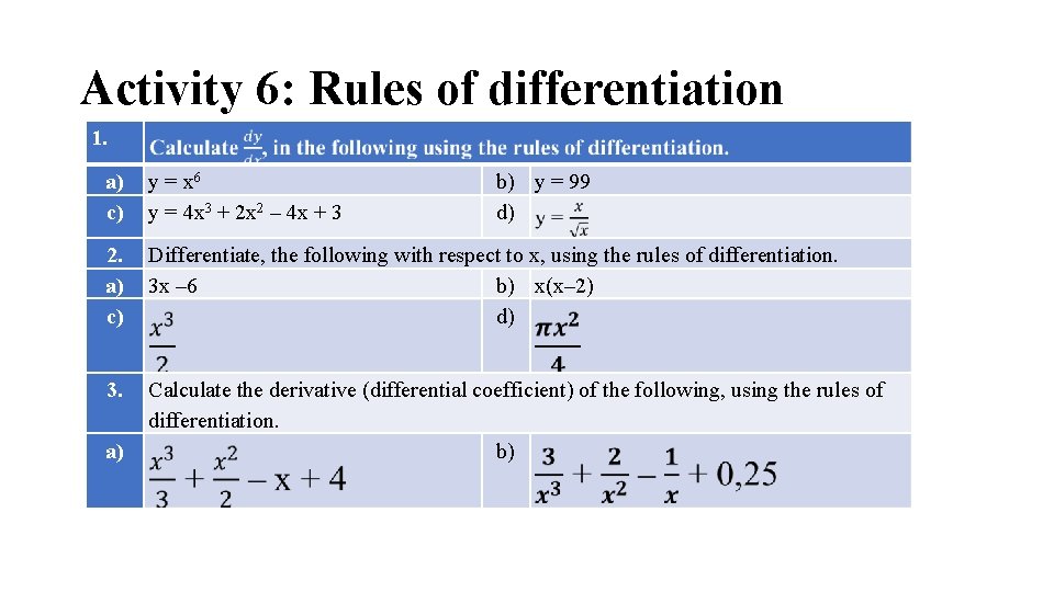
Activity 6: Rules of differentiation 1. a) c) y = x 6 y = 4 x 3 + 2 x 2 – 4 x + 3 2. a) c) Differentiate, the following with respect to x, using the rules of differentiation. 3 x – 6 b) x(x– 2) d) 3. Calculate the derivative (differential coefficient) of the following, using the rules of differentiation. b) a) b) y = 99 d)

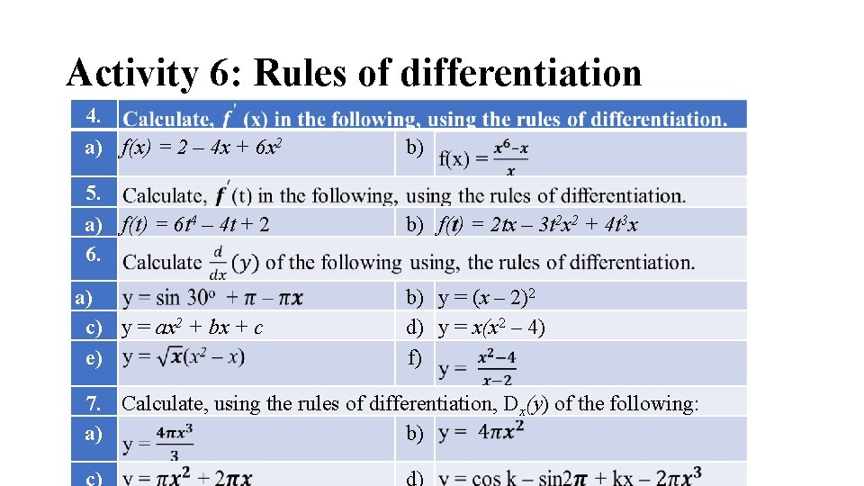
Activity 6: Rules of differentiation 4. a) f(x) = 2 – 4 x + 6 x 2 5. a) f(t) = 6 t 4 – 4 t + 2 6. a) c) y = ax 2 + bx + c e) b) b) f(t) = 2 tx – 3 t 2 x 2 + 4 t 3 x b) y = (x – 2)2 d) y = x(x 2 – 4) f) 7. Calculate, using the rules of differentiation, Dx(y) of the following: a) b) c) d)

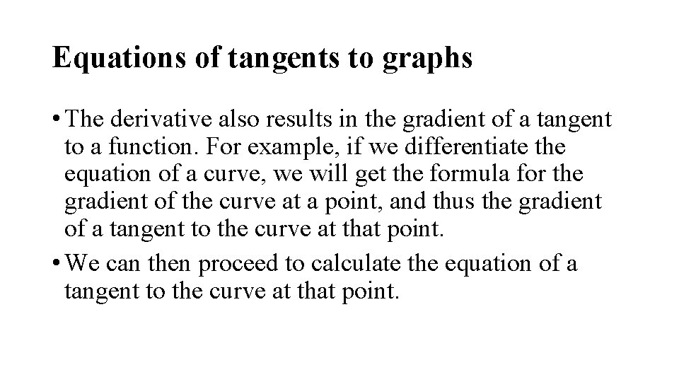
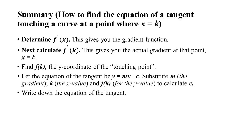
Equations of tangents to graphs • The derivative also results in the gradient of a tangent to a function. For example, if we differentiate the equation of a curve, we will get the formula for the gradient of the curve at a point, and thus the gradient of a tangent to the curve at that point. • We can then proceed to calculate the equation of a tangent to the curve at that point.

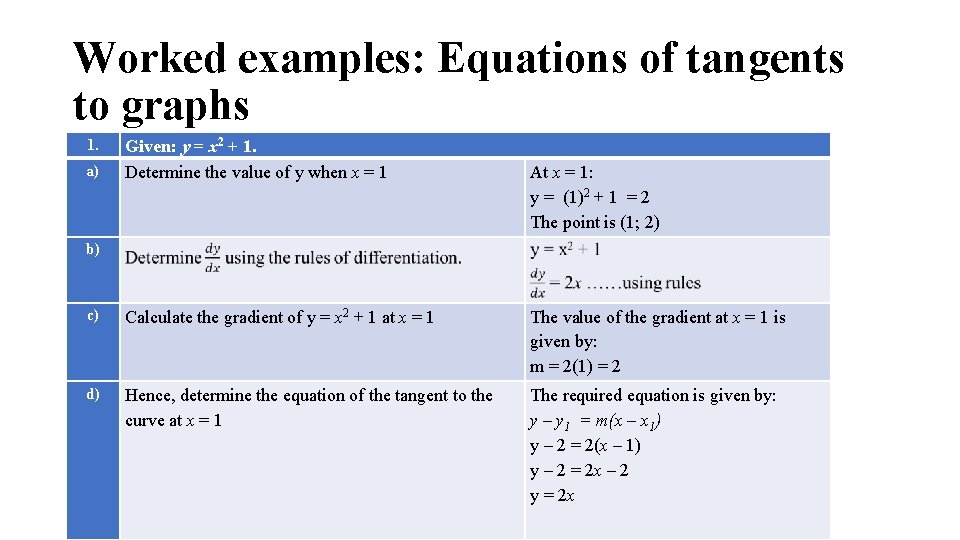
Worked examples: Equations of tangents to graphs 1. a) Given: y = x 2 + 1. Determine the value of y when x = 1 At x = 1: y = (1)2 + 1 = 2 The point is (1; 2) b) c) Calculate the gradient of y = x 2 + 1 at x = 1 The value of the gradient at x = 1 is given by: m = 2(1) = 2 d) Hence, determine the equation of the tangent to the curve at x = 1 The required equation is given by: y – y 1 = m(x – x 1) y – 2 = 2(x – 1) y – 2 = 2 x – 2 y = 2 x

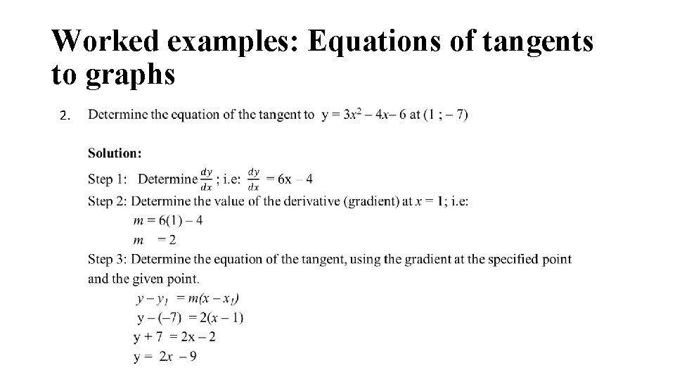
Worked examples: Equations of tangents to graphs 2.

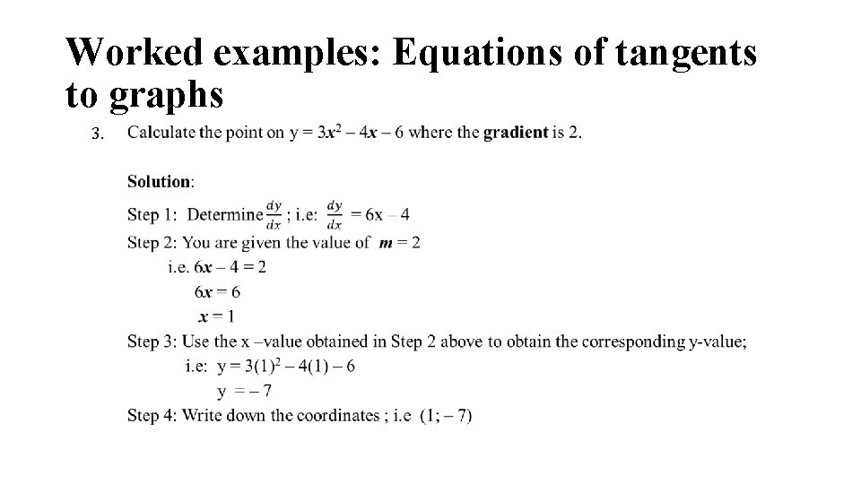
Worked examples: Equations of tangents to graphs 3.

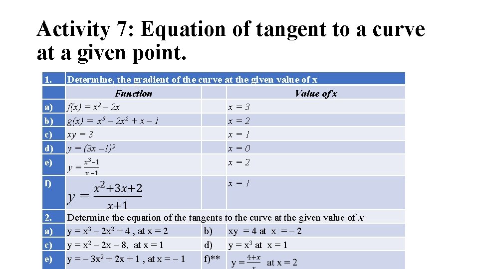
Activity 7: Equation of tangent to a curve at a given point. 1. a) b) c) d) e) f) 2. a) c) e) Determine, the gradient of the curve at the given value of x Function Value of x f(x) = x 2 – 2 x x=3 g(x) = x 3 – 2 x 2 + x – 1 x=2 xy = 3 x=1 y = (3 x – 1)2 x=0 x=2 x=1 Determine the equation of the tangents to the curve at the given value of x y = x 3 – 2 x 2 + 4 , at x = 2 b) xy = 4 at x = – 2 y = x 2 – 2 x – 8, at x = 1 d) y = x 3 at x = 1 y = – 3 x 2 + 2 x + 1 , at x = – 1 f)**

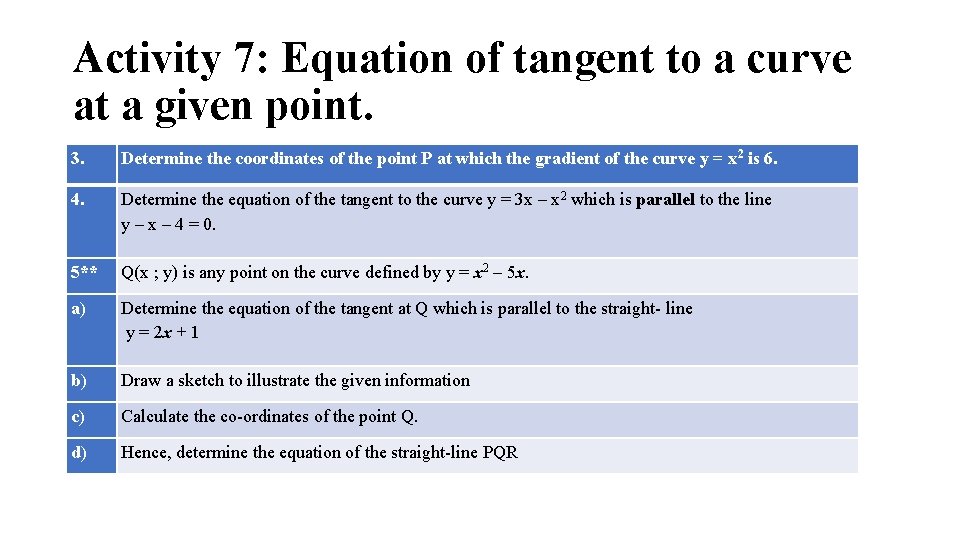
Activity 7: Equation of tangent to a curve at a given point. 3. Determine the coordinates of the point P at which the gradient of the curve y = x 2 is 6. 4. Determine the equation of the tangent to the curve y = 3 x – x 2 which is parallel to the line y – x – 4 = 0. 5** Q(x ; y) is any point on the curve defined by y = x 2 – 5 x. a) Determine the equation of the tangent at Q which is parallel to the straight- line y = 2 x + 1 b) Draw a sketch to illustrate the given information c) Calculate the co-ordinates of the point Q. d) Hence, determine the equation of the straight-line PQR

Summary (How to find the equation of a tangent touching a curve at a point where x = k) •

Sketching of cubic functions

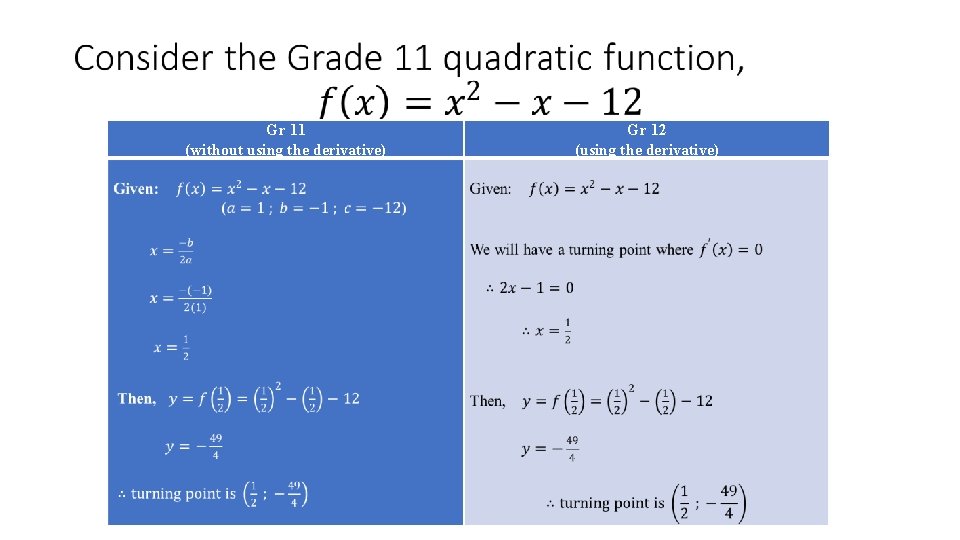
Gr 11 (without using the derivative) Gr 12 (using the derivative)

Maximum / Minimum values

Maximum / minimum values

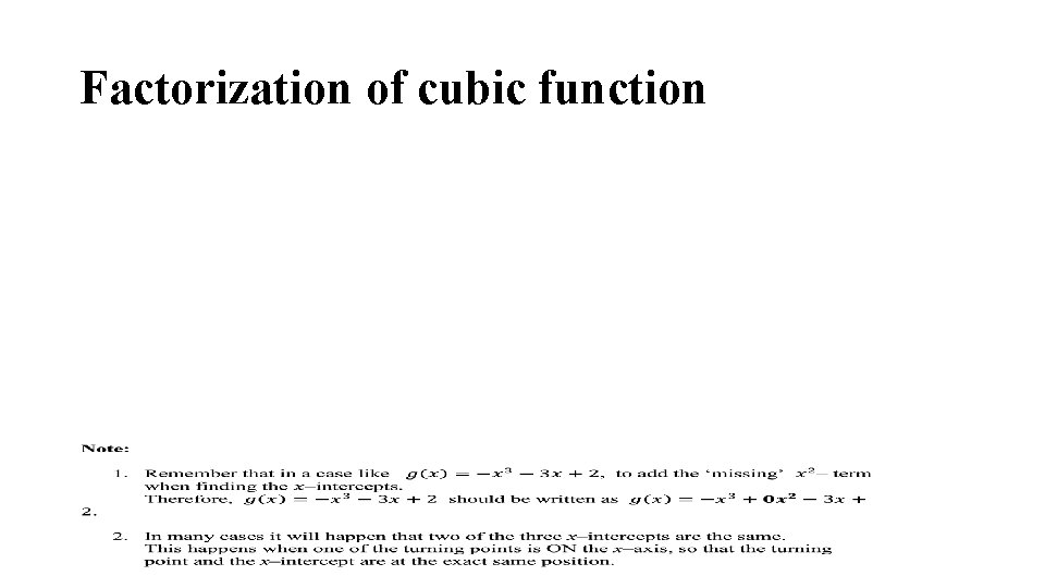
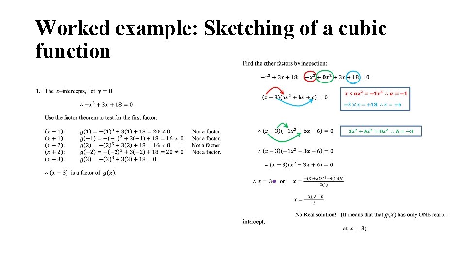
Factorization of cubic function

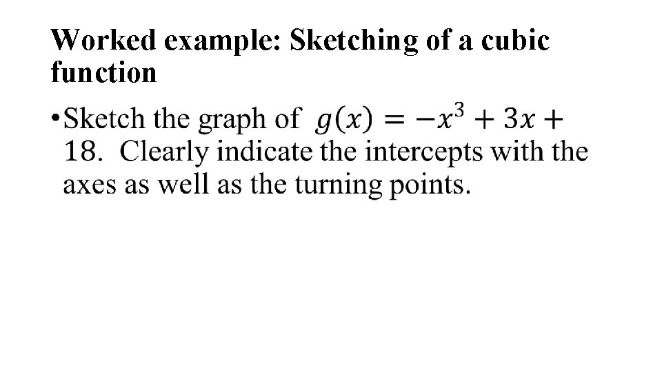
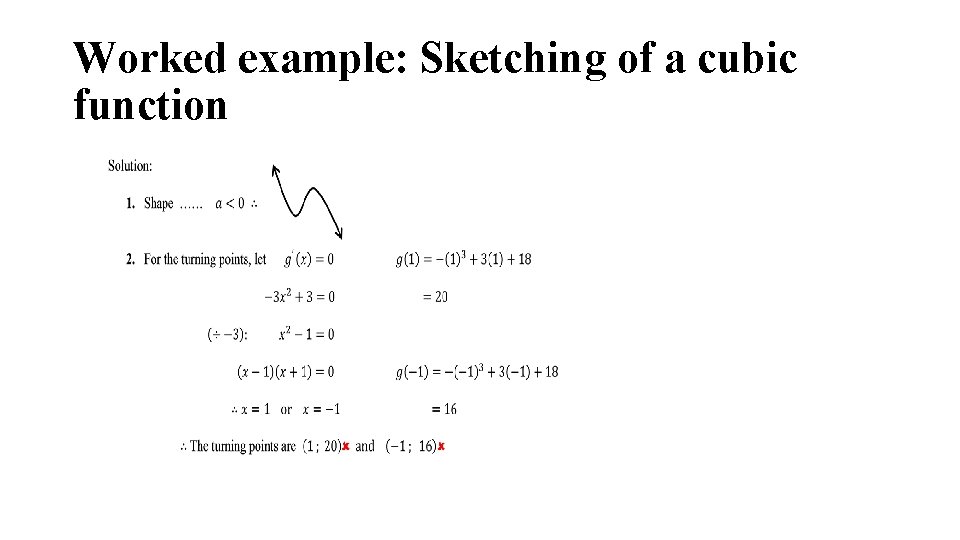
Worked example: Sketching of a cubic function •

Worked example: Sketching of a cubic function

Worked example: Sketching of a cubic function

Worked example: Sketching of a cubic function

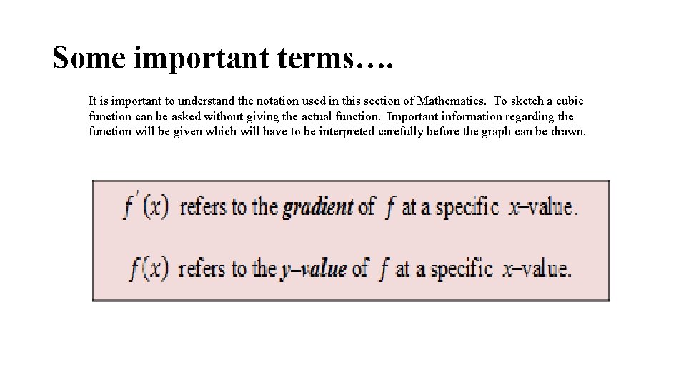
Some important terms…. It is important to understand the notation used in this section of Mathematics. To sketch a cubic function can be asked without giving the actual function. Important information regarding the function will be given which will have to be interpreted carefully before the graph can be drawn.

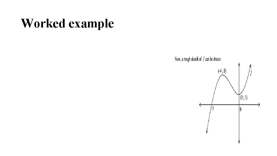
Worked example

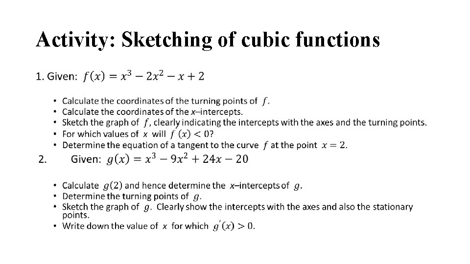
Activity: Sketching of cubic functions •

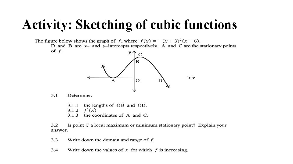
Activity: Sketching of cubic functions

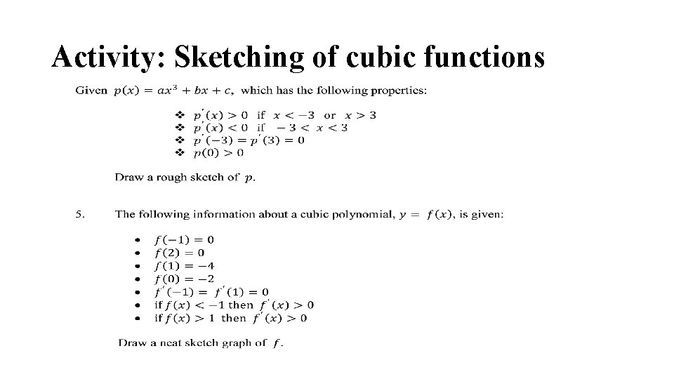
Activity: Sketching of cubic functions

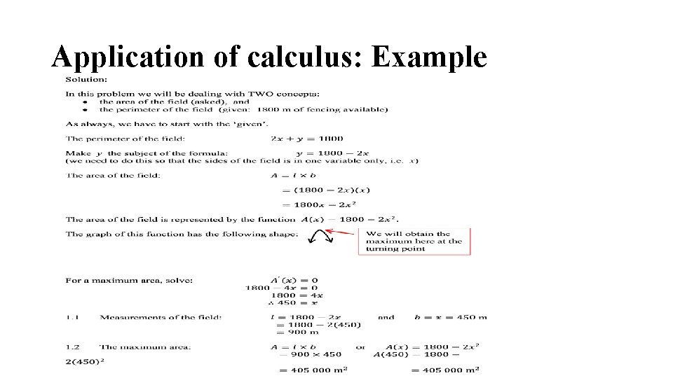
Application of calculus: Example

Application of calculus: Example

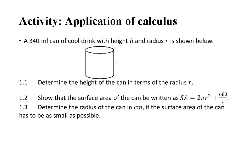
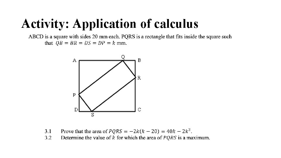
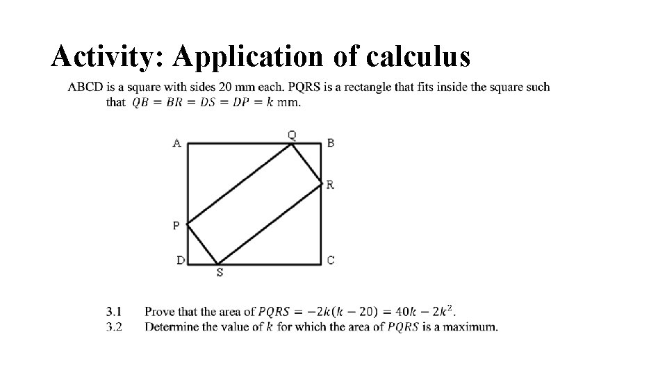
Activity: Application of calculus •

Activity: Application of calculus

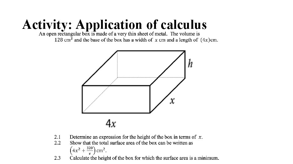
Activity: Application of calculus

Activity: Application of calculus

Calculus of motion

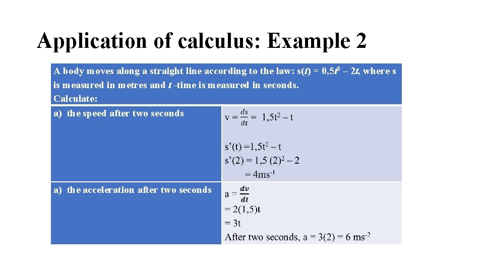
Application of calculus: Example 2 A body moves along a straight line according to the law: s(t) = 0, 5 t 3 – 2 t, where s is measured in metres and t -time is measured in seconds. Calculate: a) the speed after two seconds a) the acceleration after two seconds

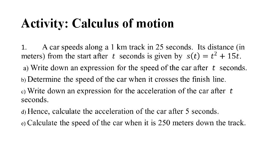
Activity: Calculus of motion •

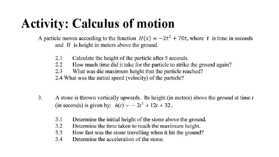
Activity: Calculus of motion

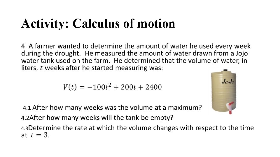
Activity: Calculus of motion •