Design of High Performance Internet Routers Dept of

Design of High Performance Internet Routers (高效能網際網路路由器設計) 張燕光 資訊 程學系 Dept. of Computer Science & Information Engineering, 國立成功大學 National Cheng Kung University 1

Outline Introduction IP lookup review (1 -D packet classification) Data structures for IP lookups Binary prefix search Layered search trees 5 -D packet classification Openflow (Software Defined Network, SDN) 12 -D packet classification Conclusion 成功大學資訊 程系 CIAL 實驗室 2

Internet: Mesh of Routers The Internet Core Edge Router Campus Area Network 成功大學資訊 程系 CIAL 實驗室 3

RFC 1812: Requirements for IPv 4 Routers Must perform an IP datagram forwarding decision (called forwarding, routing lookup, or IP lookup, longest prefix match) Must send the datagram out to the appropriate interface (called switching) 成功大學資訊 程系 CIAL 實驗室 4

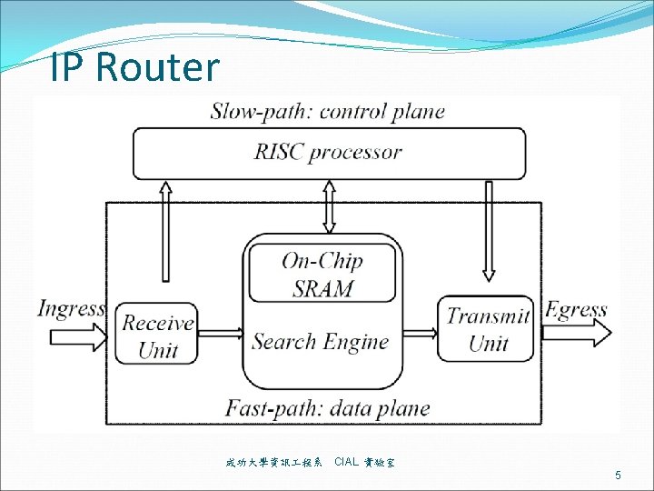
Search Engine H E A D E R Incoming Packet Dstn Addr Forwarding Engine Next Hop Computation Next Hop Forwarding Table Dstn-prefix Next Hop ------- Unicast destination address based lookup 成功大學資訊 程系 CIAL 實驗室 6

IPv 4 Addresses 32 -bit addresses Dotted quad notation: e. g. 12. 33. 32. 1 Can be represented as integers on the IP number line [0, 232 -1]: a. b. c. d denotes the integer: (a*224+b*216+c*28+d) 0. 0 IP Number Line 成功大學資訊 程系 255 CIAL 實驗室 7

IPv 6 Addresses 128 -bit addresses 成功大學資訊 程系 CIAL 實驗室 8

Example Forwarding Table P 1 P 2 P 3 P 4 Prefix 111* 1010* 10101 Next-hop H 1 H 2 H 3 H 4 Longest prefix match(LPM), not exact match Properties: prefixes are either disjoint or enclosing (one completely covers another) Prefix enclosure makes (1) sorting prefixes and (2) binary searching prefixes difficult. So, trie based schemes emerge naturally 成功大學資訊 程系 CIAL 實驗室 9

Data Structures for IP lookups 成功大學資訊 程系 CIAL 實驗室 10

Prefix properties Disjoint prefixes: Two prefixes are said to be disjoint if they do not share any address. Prefix enclosure: A = bn-1…bj…bi* and B = bn-1…bj* and j > i. Prefix A is enclosed by B (B A) since the IP address space covered by A is a subset of that covered by B, where is the enclosure operator. A special case of overlapping. Prefix comparison The inequality 0 < * < 1 is used to compare two prefixes in the ternary representation of prefixes. 成功大學資訊 程系 CIAL 實驗室 11

Prefix properties The most specific prefixes (MSP): The prefixes that do not cover any others. Disjoint, so can be put in an array for binary search Grouping prefixes in layers based on MSP. 6 -7 layers for IPv 4 tables 4 4 3 1 1 3 3 2 2 2 1 1 成功大學資訊 程系 5 1 1 3 2 2 1 1 CIAL 實驗室 12

Prefix Enclosure property Database (year-month) AS 6447 (2000 -4) AS 6447 (2002 -4) AS 6447 (2005 -4) number of prefixes 79, 530 124, 798 163, 535 Level-1 prefixes 73, 891(92. 9%) 114, 745 (91. 9%)150, 245 (91. 9%) Level-2 prefixes 4, 874 (6. 1%) 8, 496 (6. 8%) 11, 135 (6. 8%) Level-3 prefixes 642 (0. 8%) 1, 290 (1%) 1, 775 (1. 1%) Level-4 prefixes 104 (0. 1%) 235 (0. 2%) 329 (0. 2%) Level-5 prefixes 17 29 45 Level-6 prefixes 2 3 6 成功大學資訊 程系 CIAL 實驗室 13

Prefix Enclosure property Database (year-month) AS 6447 (2012 -2) AS 6447 (2014 -10) AS 6447 (2016 -5) # of prefixes Level-0 prefixes Level-1 prefixes Level-2 prefixes Level-3 prefixes Level-4 prefixes Level-5 prefixes Level-6 prefixes Level-7 prefixes Level-8 prefixes 407, 217 532, 089 642, 137 367, 980 (90. 4%) 478, 577 (89. 9%) 32, 620 (8%) 44, 171 (8. 3%) 571, 816 (89%) 57, 007 (8. 9%) 5, 353 (1. 3%) 7, 402 (1. 4%) 10, 271 (1. 6%) 997 (0. 2%) 1, 506 (0. 3%) 2, 262 (0. 4%) 210 337 581 38 73 14 21 43 5 2 13 0 0 1 成功大學資訊 程系 CIAL 實驗室 14

Prefix Enclosure property 1 -level pushing Database (year-month) # of prefixes AS 6447 (2000 -4) 397, 513 AS 6447 (2002 -4) 516, 803 Level-0 prefixes 371, 845 (93. 5%) 483, 828 (93. 6%) AS 6447 (2005 -4) 619, 087 578, 252 (93. 4%) Level-1 prefixes 23, 404 (5. 9%) 30, 252 (5. 9%) 37, 308 (6%) Level-2 prefixes 2, 115 (0. 5%) 2, 527 (0. 5%) 3, 262 (0. 5%) Level-3 prefixes 141 188 249 Level-4 prefixes 8 8 16 成功大學資訊 程系 CIAL 實驗室 15

Prefix Enclosure property Layer distribution 成功大學資訊 程系 CIAL 實驗室 16

Number Prefix properties Prefix length 成功大學資訊 程系 CIAL 實驗室 17

Prefix Forwarding table example Prefix Next-hop P 1 111* H 1 P 2 10* H 2 P 3 1010* H 3 P 4 10101 H 4 P 1 is disjoint from the other three prefixes. P 2 P 3 P 4 Longest prefix match(LPM), not exact match enclosure makes (1) sorting prefixes and (2) binary searching prefixes difficult So, trie based schemes emerge naturally 成功大學資訊 程系 CIAL 實驗室 18

Binary Trie (Radix Trie) Lookup 10111 P 1 111* H 1 P 2 10* H 2 P 3 1010* H 3 P 4 10101 H 4 A 1 C P 2 G P 3 next-hop-ptr (if prefix) right-ptr left-ptr B 1 0 1 D Add P 5=1110* 1 E 0 1 Trie node 0 P 4 成功大學資訊 程系 H P 5 P 1 F I CIAL 實驗室 19

Binary Trie: Leaf Pushing P 1 111* H 1 P 2 10* H 2 P 3 1010* H 3 P 4 10101 H 4 P 5 1110 H 5 P 2 Disjoint, but duplication P 3 P 5 P 1 P 4 成功大學資訊 程系 CIAL 實驗室 20

Prefix formats (representation) Length format: bn-1…b 0/l (l is prefix length) In IPv 4, d 3. d 2. d 1. d 0/l , 140. 116. 82. 36/24. Mask format: bn-1…b 0/mn-1…m 0 (prefix length is l) mj = 1 for all n – 1 j n – l, and mj =0 otherwise. d 3. d 2. d 1. d 0/ m 3. m 2. m 1. m 0, 140. 116. 82. 36/1. . . 10000 Ternary format: bn-1…bn-l+1*…* (prefix length is l) 140. 0/8 = 10001100* 成功大學資訊 程系 CIAL 實驗室 21

A New Prefix format (n+1)-bit format: bn-1…bn-l 10… 0 (l is prefix len) for the prefix bn-1…bn-l* of length l in ternary format, there is one trailing ‘ 1’ followed by n – l 0’s. or symmetrically (n+1)-bit format: bn-1…bn-l 01… 1 for the prefix bn-1…bn-l* of length l in ternary format, there is one trailing ‘ 0’ followed by n – l 1’s. 成功大學資訊 程系 CIAL 實驗室 22

5 -bit Prefixes: bn-1…bn-l 10… 0 ***** 00*** 0 0 0 * * 0 0 0 0 1 0 0 0 0 1 1 11*** 0 0 0 1 0 * 0 0 0 1 1 0 0 0 1 0 0 0 1 1 1 0 1 * 1 1 1 0 0 0 6 -bit binary address space 000000 is not used 成功大學資訊 程系 1 1 1 0 0 0 1 1 1 * * 1 1 1 1 0 1 1111111 0001111 0110011 1010101 CIAL 實驗室 23

5 -bit Prefixes: bn-1…bn-l 01… 1 ***** 00*** 0 0 0 * * 0 0 0 0 1 0 0 0 1 0 0 0 0 0 1 1 11*** 0 0 0 1 0 * 0 0 0 1 1 0 0 0 1 0 0 0 1 1 1 0 1 * 1 1 1 0 0 0 1 6 -bit binary address space 111111 is not used 成功大學資訊 程系 11 11 01 10 10 10 1 1 1 * * 1 1 1 1 0 1 111111 000111 011001 101010 CIAL 實驗室 24

Prefix: a special case of Range format: [b, e], b and e are begin and endpoints Prefixes are special cases of ranges. Prefix bn-1…bn-l* of length l is the range of addresses from bn-1…bn-l 0… 0 to bn-1…bn-l 1… 1, denoted as [bn-1…bn-l 0… 0, bn-1…bn-l 1… 1] or bn-1…bn-l*. Overlapping: Two ranges are overlapping if they are not disjoint. Partially overlapping: Two ranges are partially overlapping if they are neither disjoint nor enclosing. So, two prefixes can not be partially overlapped The source/destination port fields of rule tables for packet classification are ranges. 成功大學資訊 程系 CIAL 實驗室 25

Elementary Intervals for Ranges Definition: Let the set of k elementary intervals constructed from a set R of ranges in the address space of 0 … N – 1 be X = {Xi | Xi = [ei, fi], for i = 1 to k}. X must satisfy the following: 1) e 1 = 0 and fk = N – 1, 2) fi = ei+1 – 1 for i = 1 to k – 1, 3) all addresses in Xi are covered by the same subset of R (called the range matching set of Xi) denoted by EIi, and 4) EIi+1, for i = 1 to k – 1. 成功大學資訊 程系 CIAL 實驗室 26

Elementary Intervals for Ranges Graphical view EI 1 EI 2 EI 3 P 1 [0 , 15] {P 1} {P 1, P 3} {P 1} P 2 [16, 31] X 1 X 2 X 3 P 3 [4 , 7] [0, 3] [4, 7] [8, 15] P 4 [32, 63] P 1 P 3 P 5 [22, 23] EI 7 EI 8 EI 9 P 6 [48, 63] {P 4, P 9} {P 4, P 6, P 7 [48, 51] X 7 X 8 } [32, 39] [40, 47] X 9 P 8 [55, 55] [48, 51] P 9 [32, 39] P 4 P 9 EI 4 EI 5 EI 6 {P 2} {P 2, P 5} {P 2} X 4 X 5 X 6 [16, 21] [22, 23] [24, 31] P 5 EI 10 EI 11 EI 12 {P 4, P 6} {P 4, P 6, P 8 {P 4, P 6} X 10 } X 12 [52, 54] X 11 [56, 63] [55, 55] P 6 P 7 成功大學資訊 程系 P 2 P 8 CIAL 實驗室 27

Elementary Intervals for Ranges ID Prefix Range P 1 P 2 P 3 P 4 P 5 P 6 P 7 P 8 P 9 000000/2 010000/2 000100/4 100000/1 010110/5 110000/2 110000/4 110111/6 100000/3 [0, 15] [16, 31] [4, 7] [32, 63] [22, 23] [48, 63] [48, 51] [55, 55] [32, 39] 成功大學資訊 程系 Minus-1 start finish 15 15 31 3 7 31 21 23 47 47 51 54 55 31 39 Traditional start finish 0 15 16 31 4 7 32 63 22 23 48 63 48 51 55 55 32 39 CIAL 實驗室 28

Segment Tree 23 w 7 y 47 P 1 u 3 15 v 31 z P 4 P 6 g q 54 15 P 3 X 1 X 2 [0, 3] [4, 7] P 1 X 3 [8, 15] leaf node P 2 h 21 P 2 P 4 r 39 X 6 [24, 31] P 5 X 4 X 5 [16, 21][22, 23] 成功大學資訊 程系 P 9 51 P 7 s 55 t P 8 X 7 X 8 X 9 X 10 X 11 X 12 [32, 39] [40, 47] [48, 51] [52, 54] [55, 55] [56, 63] CIAL 實驗室 29

Hash Table Narrowing down the search space. Index = Hash_function(key)%m, where key may be the first k bits of IP addresses and m is the size of the hash table. Perfect hash: no collision Minimal perfect hash: A perfect hash, where the size of its hash table is k for k different hashing keys. P 1 111* H 1 P 2 10* H 2 P 3 1010* H 3 P 4 10101 H 4 P 5 1110 H 5 成功大學資訊 程系 CIAL 實驗室 30

Hash Table Difficulties: prefixes and ranges can not be used as the keys of the hash functions directly. Array of m elements H(k 1)%m k 1 k 2 H(k 2)%m collision 成功大學資訊 程系 CIAL 實驗室 31

Hash Table Prefix bn-1…b 0/l = bn-1…bn-l 0… 0/l Hash(bn-1…bn-l 0… 0, l) = h Store bn-1…bn-l 0… 0/l in bucket h of the hash table When Input IP = bn-1…b 0 We have to search multiple times as follows Hash(bn-1…bn-i 0… 0, i) for i = 1 to max_length 成功大學資訊 程系 CIAL 實驗室 32

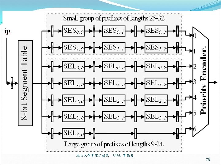
Hash Table: 8 -bit Segmentation table A 8 -bit segmentation table is usually used for IPv 4 forwarding tables because there is no prefix of length shorter than 8. Array of 256 elements 0 H(prefix)%256 (MSB 8 bits of prefix) Prefix: 0. x. y. z 1 Prefixes with the same first 8 MSB bits Maybe empty set 255 成功大學資訊 程系 CIAL 實驗室 33

Hash Table: 16 -bit Segmentation table Prefixes of length <= 16 must be stored properly. For example, duplicate 0. 0. b. c/15 into buckets 0 and 1 or store the port of 0. 0. b. c/15 into elements 0 and 1. Put them into another set (good for update but need to search two sets in the worst case). Array of 216 elements 0 H(prefix)%216 (MSB 16 bits of prefix) Prefix: 0. 0. y. z 1 Prefixes with the same first 16 MSB bits Maybe empty set Prefixes of length 16 成功大學資訊 程系 216 -1 CIAL 實驗室 34

Hash Table: Compression Since there are many empty elements in the segmentation table, we can use bitmap to compress the segmentation table. 216 -Bitmap containing M 1’s Array of M elements 0 1 1 0 0. . . 0 1 1 0 0 1 1 Prefix: 0. 0. y. z Prefix: 0. 1. y. z Prefixes with the same first 16 MSB bits Must be non-empty M-1 成功大學資訊 程系 CIAL 實驗室 35

Field Split Bit Vector Multi-match packet classification is a critical function in network intrusion detection systems (NIDS), where all matching rules for a packet need to be reported. Most of the previous work is based on ternary content addressable memories (TCAMs) which are expensive and are not scalable with respect to clock rate, power consumption, and circuit area. National Cheng Kung University CSIE Computer & Internet Architecture Lab 36

Field Split Bit Vector The proposed architecture is called field-split parallel bit vector (FSBV) where some header fields of a packet are further split into bit-level subfields. National Cheng Kung University CSIE Computer & Internet Architecture Lab 37

Field Split Bit Vector (FSBV) Stride=1 R 1 F[4]= Rule Field F R 1 10011 R 2 101*0 R 3 01001 R 4 1**00 F[3]= FSBV F[2]= F[1]= F[0]= R 2 R 3 R 4 0 1 0 1 0 1 Field-split bit vector generation and classification operation Computer & Internet Architecture Lab CSIE, National Cheng Kung University 38

Field Split Bit Vector (FSBV) Stride=1 R 1 F[4]= Rule Field F R 1 10011 R 2 101*0 R 3 01001 R 4 1**00 F[3]= FSBV F[2]= F[1]= F[0]= R 2 R 3 R 4 0 1 1 0 0 1 1 Field-split bit vector generation and classification operation Computer & Internet Architecture Lab CSIE, National Cheng Kung University 39

Field Split Bit Vector (FSBV) Stride=1 F[4]= Rule Field F R 1 10011 R 2 101*0 R 3 01001 R 4 1**00 F[3]= FSBV F[2]= F[1]= F[0]= R 1 R 2 1 1 0 0 0 1 R 3 R 4 0 1 0 1 1 1 0 0 1 Field-split bit vector generation and classification operation Computer & Internet Architecture Lab CSIE, National Cheng Kung University 40

Field Split Bit Vector (FSBV) Stride=1 F[4]= Rule Field F R 1 10011 R 2 101*0 R 3 01001 R 4 1**00 F[3]= FSBV F[2]= F[1]= F[0]= R 1 R 2 R 3 1 1 0 0 0 1 0 R 4 0 1 0 1 1 1 1 0 1 0 1 Field-split bit vector generation and classification operation Computer & Internet Architecture Lab CSIE, National Cheng Kung University 41

Field Split Bit Vector (FSBV) Stride=1 F[4]= Rule Field F R 1 10011 R 2 101*0 R 3 01001 R 4 1**00 F[3]= FSBV F[2]= F[1]= F[0]= R 1 R 2 R 3 R 4 1 1 0 1 0 1 1 0 0 1 1 1 0 0 1 0 0 1 Field-split bit vector generation and classification operation Computer & Internet Architecture Lab CSIE, National Cheng Kung University 42

Field Split Bit Vector (FSBV) Stride=1 F[4]= Rule Field F R 1 10011 R 2 101*0 R 3 01001 R 4 1**00 F[3]= FSBV F[2]= F[1]= F[0]= R 1 R 2 R 3 R 4 0 0 0 1 1 1 0 0 1 1 0 1 0 1 0 0 1 1 1 0 0 1 0 1 1 1 0 Field-split bit vector generation and classification operation Computer & Internet Architecture Lab CSIE, National Cheng Kung University 43

Field Split Bit Vector (FSBV) Stride=1 F[4]= Rule Field F R 1 10011 R 2 101*0 R 3 01001 R 4 1**00 F[3]= FSBV F[2]= F[1]= F[0]= Incoming packet: F = 10110 R 1 R 2 R 3 R 4 0 0 0 1 1 1 0 1 1 0 1 0 1 1 1 0 1 0 1 0 0 1 1 0 0 1 0 1 0 1 1 1 0 Field-split bit vector generation and classification operation Computer & Internet Architecture Lab CSIE, National Cheng Kung University 44

Field Split Bit Vector (FSBV) Stride=1 F[4]= Rule Field F R 1 10011 R 2 101*0 R 3 01001 R 4 1**00 F[3]= FSBV F[2]= F[1]= F[0]= Incoming packet: F = 10110 R 1 R 2 R 3 R 4 0 0 0 1 1 1 0 1 1 0 1 0 1 1 1 0 1 0 0 1 1 0 0 1 0 1 0 1 1 1 0 0 1 Multimatch Result Match R 2 Field-split bit vector generation and classification operation Computer & Internet Architecture Lab CSIE, National Cheng Kung University 45

Stride Bit Vector (Stride. BV) Stride Bit Vector also called Stride. BV which is extended from FSBV as we mentioned before. If using the FSBV to apply for total field of traditional packet classification, the system will result 104 stages in pipeline on FPGA, and this will cause the latency of system too long. Stride. BV will reduce the number of stages used for the system by using multiple bits (stride size = k) than one bit designed in FSBV. National Cheng Kung University CSIE Computer & Internet Architecture Lab 46

Stride Bit Vector (Stride. BV) stride =2 l Stride bit vector generation and classification operation Rule Field F Stride. BV (stride size = 2) 1101 *1*0 001* **** Input packet A = 0110 0 A= 1 1 0 F[1] 00 01 10 11 1 1 0 0 0 1 1010 F[0] 00 01 10 11 1 1 0 0 1 0 0 National Cheng Kung University CSIE Computer & Internet Architecture Lab 1110 47

Stride Bit Vector (Stride. BV) stride =4 l Stride bit vector generation and classification operation Rule Field F Stride. BV (stride size = 4) 1101 *1*0 001* **** Input packet A = 0110 0 A= 1 1 0 F[0] 0000 0001 0010 0011 0100 0101 0110 0111 1000 1001 1010 1011 1100 1101 1110 1111 1 1 1 1 0 0 1 1 0 0 0 0 1 0 1 0 0 0 0 0 1 0 0 National Cheng Kung University CSIE Computer & Internet Architecture Lab 1010 48

Metrics for Lookup Algorithms High Speed (ex. 40 Gbps/40 -byte=128 m packets/sec) Small storage (ex. Cache or On-Chip memory) Low update time Ability to handle large routing tables Flexibility in implementation Low preprocessing time IPv 6 成功大學資訊 程系 CIAL 實驗室 49

Survey: IP Lookups M. A. Ruiz-Sanchez, E. W. Biersack, and W. Dabbous, “Survey and taxonomy of IP address lookup algorithms, ” IEEE Network, vol. 15, pp. 8– 23, March 2001. Schemes for optimizing search speed Multibit tries Two-level multibit trie, 16 -16, 24 -8 Binary range search (endpoint) Binary search on prefix length Binary prefix search Binomial Spanning tries based on Hamming and Golay perfect codes FPGA pipelined implementation (over 100 Gbps) 成功大學資訊 程系 CIAL 實驗室 50

Existing IP lookup schemes Schemes for optimizing memory requirement Small forwarding table (SFT): compressed 16 -8 -8 trie Level compressed (LC) trie Huang ‘s compressed 16 -x (C-16 -x) Compressed 8 -8 -8 -8 trie using minimal perfect hashing function Hierarchical endpiont tree (01** 0100 and 1000) Tree bitmap (compressed 4 -4 -4 -4 -4 trie) Memory optimized multibit tries with dynamic programming 成功大學資訊 程系 CIAL 實驗室 51

Existing IP lookup schemes Schemes for optimizing update speed (log N) Binary tree on binary tree scheme (PBOB), Priority search tree scheme (PST), Collection of red-black tree schemes (CRBT) Most Specific Prefix Tree (MSPT) Multigroup Most Specific Prefix Tree (MG-MSPT) Dynamic segment tree (DST), extending binary range search Multiway range tree (MRT) Prefix in B-Tree (PIBT) Dynamic Multiway Segment Tree (DMST) 成功大學資訊 程系 CIAL 實驗室 52

Existing IP lookup schemes Schemes for optimizing IPv 6 Not really Some dual stack (IPv 4/IPv 6) papers 128 -bit IPv 6 addresses 32 -bit vs. 64 -bit CPUs or Memory bandwidth Initial results: binary search based schemes are better than trie based schemes 成功大學資訊 程系 CIAL 實驗室 53

Binary Trie (Radix Trie) Lookup 10111 P 1 111* H 1 P 2 10* H 2 P 3 1010* H 3 P 4 10101 H 4 A 1 C P 2 G P 3 next-hop-ptr (if prefix) right-ptr left-ptr B 1 0 1 D Add P 5=1110* 1 E 0 1 Trie node 0 P 4 成功大學資訊 程系 H P 5 P 1 F I CIAL 實驗室 54

Existing Binary Range Search Traditional Endpoint: [e, f] e and f. 成功大學資訊 程系 CIAL 實驗室 55

Proposed Binary Range Search Proposed Endpoint: minus-1 -endpoint range [e, f] e – 1 and f. 成功大學資訊 程系 CIAL 實驗室 56

Binary prefix search Definition 1 (Prefix comparison): The inequality 0 < * < 1 is used to compare two prefixes in the ternary format. 成功大學資訊 程系 CIAL 實驗室 57

Binary prefix search Directly performing a binary search on the list of sorted prefixes may encounter a failure: Dst = 01011000 2 4 3 Correct match 成功大學資訊 程系 1 Failed match CIAL 實驗室 58

Binary prefix search Enclosure relationship between prefixes results in the search failure Generate some auxiliary prefixes that inherit the routing information of the original LPM (e. g. , F) and put them where the binary search operations can find them. ex. auxiliary prefix 01011000. Therefore, it is feasible to split prefix F into two parts such that both sides of prefix O are covered. 成功大學資訊 程系 CIAL 實驗室 59

Binary prefix search The full tree expansion splits the enclosure prefixes into many longer prefixes (leaf pushing). Auxiliary prefix merges Many auxiliary prefixes may inherit the same routing information of a common enclosure prefix. These prefixes can be merged into one. The merge operation is defined as follows. Prefix merge: The prefix obtained by merging a set of consecutive prefixes is the longest common ancestor (LCA) of these consecutive prefixes in the binary trie. 成功大學資訊 程系 CIAL 實驗室 60

Binary prefix search The full tree expansion F 3=01011000 成功大學資訊 程系 CIAL 實驗室 61

Binary prefix search The full tree after the merge operations F 3=01011000 成功大學資訊 程系 CIAL 實驗室 62

Performance: Search Speed 成功大學資訊 程系 CIAL 實驗室 63

Performance: Search Speed 成功大學資訊 程系 CIAL 實驗室 64

Table 3: For 120, 635 prefixes and multiway assumes 64 -byte cache block. Scheme Segmentation Statistics Ref. Memory Original table Binary trie BSD trie Compressed 16 -x LC trie SFT N/A 16 -bit segmentation 65535 entries (4 byte each) # of prefixes: 120, 635 (45 bits each) # of nodes: 320, 478 (7 bytes each) # of nodes: 222, 334 (8 bytes each) Base array: 427 KB Compressed Bit-map: 427 KB CNHA: 37. 9 KB 662. 7 KB 8/32 2, 447 KB 8/26 1, 993 KB # of prefixes: 232, 887 (6 bytes each) # of prefixes: 217, 146 (4 bytes each) # of blocks: 71, 034 (64 bytes each) # of prefixes: 145, 737 (5 bytes each) # of prefixes: 117, 968 (3 bytes each) # of blocks: 11, 175 (64 bytes each) 1/6 1/4 1/5 1/4 1/3 N/A 1/3 1, 147 KB # of nodes: 259, 371 (4 bytes each) 1/5 2, 859 KB Branch factor: 16 Base vector: 110, 679 (16 bytes each) Fill factor: 0. 5 Prefix vector: 9, 927 (12 bytes each) Next Hop vector: 255 (4 bytes each) # of segments (avg # of prefixes per segment) level-1 pointers: Sparse: 2, 765 (2. 9) 1/12 649. 9 KB Dense: 4, 300 (25. 5) 13, 317 Very dense: 586 (91. 7) level-2 pointers: Maptable: 5. 3 K 461 Base array: 2 K (4 bytes each) Code Word array: 8 K Binary range No segmentation Binary range 16 -bit segmentation Multiway range 16 -bit segmentation Binary prefix No segmentation Binary prefix 16 -bit segmentation Multiway prefix 16 -bit segmentation 成功大學資訊 程系 1, 365 KB 1, 104 KB 4, 695 KB 646 KB 601 KB 954. 4 KB CIAL 實驗室 65

Goal of hardware approaches Pipeline architecture to achieve throughput of over 100 Gbps The most popular design is based on multibit trie Advantages Simple Bubble instruction to perform updates Disadvantages Unbalanced memory among stages (solvable) Memory requirement is too large to fit in the on-chip memory of hardware device such as FPGA 成功大學資訊 程系 CIAL 實驗室 66

Multibit trie pipeline Pipeline registers 67 成功大學資訊 程系 CIAL 實驗室 67

References for existing pipelines Ring - ISCA-2005 -A Tree Based Router Search Engine Architecture with Single Port Memories SDP - SIGCOMM-2005 -Dynamic Pipelining Making IPLookup CAMP - ANCS-2006 -CAMP：Fast and Efficient IP Lookup Architecture OLP - HOTI-2007 -A Memory-Balanced Linear Pipeline Architecture for Trie-based IP Lookup Bi. OLP - FCCM-2008 -A SRAM-based Architecture for Trie-based IP Lookup Using FPGA Du. PI - FPL-2008 -Scalable high-throughput SRAMbased architecture for IP-lookup using FPGA 成功大學資訊 程系 CIAL 實驗室 68

References for existing pipelines Hash - Hot. I-2008 -An Efficient Hardware-based Multi-hash Scheme for High Speed IP Lookup POLP - INFOCOM-2008 -Beyond TCAM-An SRAM based parallel multi-pipeline architecture for terabit IP lookup POLP - IPDPS-2008 -Parallel IP Lookup Using Multiple SRAMbased Pipelines Flash. Look - HPSR-2009 -Flash. Look 100 Gbps Hash-Tuned Route Lookup Architecture FPL - HPSR-2009 -Frugal IP Lookup Based on a Parallel Search p. DST - FPGA-2010 -High Throughput and Large Capacity Pipelined Dynamic Search Tree on FPGA Flash. Trie - INFOCOM-2010 -Flash. Trie- Hash-based Prefix. Compressed Trie for IP Route Lookup Beyond 100 Gbps 成功大學資訊 程系 CIAL 實驗室 69

References for existing pipelines DMST - TC-2010 -Dynamic Multiway Segment Tree for IP Lookups and the Fast Pipelined Search Engine BPFL & POLP - HPSR-2011 -FPGA implementation of lookup algorithms Shuffled Trie - ICC-2011 -Bit-Shuffled Trie IP Lookup with Multi-Level Index Tables Prefix Partitioning - TC-2011 -Scalable Tree-based Architectures for IPv 4 v 6 Lookup Using Prefix Partitioning 成功大學資訊 程系 CIAL 實驗室 70

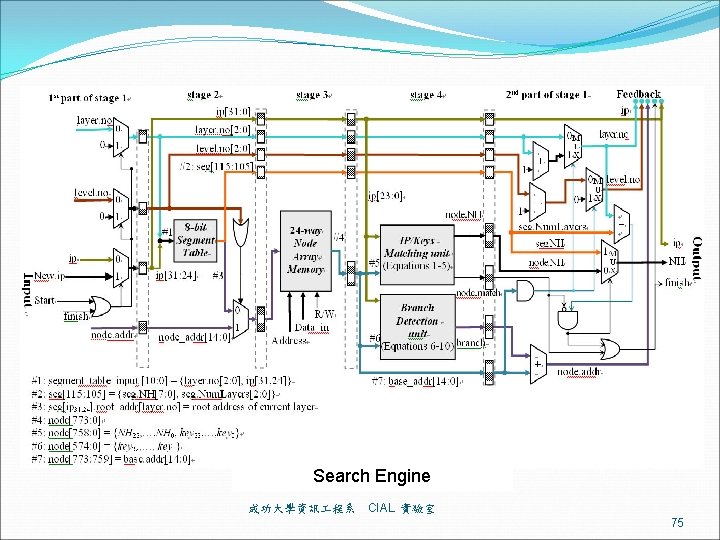
B-Tree structure 成功大學資訊 程系 CIAL 實驗室 71

B-tree structure layer 0 12 P 5 2 P 7 5 7 P 10 P 11 22 P 8 25 P 12 88 P 3 30 P 9 layer 1 4 P 4 20 P 6 72 P 1 layer 2 24 P 2 成功大學資訊 程系 CIAL 實驗室 72

B-Tree structure 成功大學資訊 程系 CIAL 實驗室 73

B-Tree structure 成功大學資訊 程系 CIAL 實驗室 74

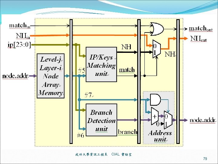
Matching unit ip and keyx are matched 成功大學資訊 程系 CIAL 實驗室 76

Branch Detection Unit 成功大學資訊 程系 CIAL 實驗室 77

Prefix Enclosure Analysis (1/2) Routing Table AS 6447 (2005 -4) AS 6447 (2009 -7) AS 6447 (2011 -5) size 163, 535 301, 552 369, 394 0 150, 245 (91. 9%) 273, 944 (90. 8%) 334, 445 (90. 5%) Layer 1 11, 135 (6. 8%) 23, 171 (7. 7%) 28, 930 (7. 8%) 2 1, 775 (1. 1%) 3, 690 (1. 2%) 4, 870 (1. 3%) 3 329 (0. 2%) 628 (0. 2%) 926 (0. 3%) 4 45 101 177 5 6 16 30 6 0 2 12 7 0 0 4 成功大學資訊 程系 CIAL 實驗室 80

Prefix Enclosure Analysis (2/2) After small push Routing Table size length AS 6447 (2005 -4) 163, 535 AS 6447 (2009 -7) 301, 552 AS 6447 (2011 -5) 355, 893 9 -24 25 -32 0 7, 071 3, 488 271, 548 5, 736 333, 034 5579 1 496 67 17, 081 28 20, 884 21 Layer 2 54 3 6 4 0 1, 488 0 88 2 成功大學資訊 程系 1, 859 0 111 0 5 CIAL 實驗室 81

Performance Comparisons Scheme Throughput Clock # of accessed Configurable Memory # of ME ratio Mpps Gbps rate nodes / search FPGA Device logic (slice) (Mbits) prefixes bits/prefix (ns) avg worst LSE Parallel LSE 1, 402 (2. 8%) 10. 9 37. 0 3. 157 3. 02 13 104. 9 24. 4 Virtex-6 301, 552 XC 6 VSX 315 T 7, 408 (15%) 10. 8 36. 8 2. 649 1 377. 5 463 (1%) 74. 9 5. 00 4. 68 6 42. 7 33. 3 Virtex-5 Original DMST [7] 11. 68 163, 574 VLX 330 T Extended 2, 778 (6%) 74. 9 5. 00 1. 0 200 Ring [1] 408 (1%) 3. 49 116. 4 2. 0 125 CAMP [11] Virtex-2 P XC 2 VP 70 528 (2%) 3. 89 129. 6 1. 3 200 30, 000 4. 00 OLP [10] 362 (1%) 3. 46 115. 2 1. 0 250 (a) Bi. OLP [12] Virtex-4 FX 140 1, 785 (3%) 9. 54 83, 662 114. 0 3. 069 1. 0 325 (a) (b) BPFL 27. 9 K LE 5. 6 18. 1 10. 35 1. 0 96. 6 [23] (19%) Stratix II 309, 000 EP 2 S 180 F 1020 C 5 6. 6 K LE (b) POLP(a) 9. 08 29. 4 9. 29 1. 0 107. 6 [23] (5%) p. DST(d) 12. 8 k Virtex-5 LX 330 7. 112 96, 000 75. 86 7. 4 1. 0 242 [44] LUTs(6. 3%) BSTrie(a) Virtex-5 749 (2%) 7. 38 321, 000 23. 0 5. 7 1. 0 175 [22] XC 5 VSX 240 T Notes: (a) the next hops are not stored in on-chip memory. (b) Instead of slices, Stratix LEs are used. (c) It is the non-cache based Bi. OLP. (d) dual-ported block RAM is used 33. 6 7. 8 120. 8 21. 9 17. 1 102 40 64 80 104 30. 9 34. 4 77. 4 56 Y. -K. Chang, F. -C. Kuo, H. -J. Kuo, C. -C. Su, "Layered. Trees: Most Specific Prefix based Pipelined Design for On-Chip IP Address Lookups", IEEE Transactions on Computers, Vol. 63, No. 12, December 2014. 成功大學資訊 程系 CIAL 實驗室 82

5 D Packet Classification performed by routers to classify the incoming packets into flows according to a set of rules If a packet matches multiple rules, the matching rule with the highest priority is returned. Typically, each rule contains five fields, Source IP address, destination IP address, source port number, destination port number, protocol type 83

A real-life classifier in five dimensions Rule Dst. IP Src. IP Dst port R 1 140. 116. 246. 69/32 140. 116. 82. 11/32 * R 2 140. 126. 53. 0/24 140. 116. 100. 157/32 80 R 3 140. 116. 247. 4/32 140. 116. 160. 0/24 > 1023 R 4 0. 0/0 * prefix Classification examples Src port * * Protocol # Action * Deny tcp Deny udp Permit * Permit range PKT Dst. IP Src. IP Dst port P 1 140. 116. 246. 69 140. 116. 82. 11 80 P 2 140. 126. 53. 10 140. 116. 100. 57 80 P 3 140. 116. 247. 4 140. 116. 160. 10 1024 Src port 1222 1233 1235 Protoc # Action tcp Deny, R 1 udp Deny, R 2 tcp Permit, R 3 84

David Taylor’s Survey (Before 2003) Exhaustive Search Decomposition Crossproducting TCAM RFC ABV Linear Search EGT Hi. Cuts Grid-of. Tries* Decision Tree FIS Trees E-TCAM Pruned Tuple Space Rectangle Search Tuple Space 85

Packet Classification David E. Taylor, Survey & Taxonomy of Packet Classification Techniques, ACM Computing Surveys, Volume 37, Issue 3, 238 -275, September 2005. Hierarchical trie, set-prunning trie, grid of trie Hierarchical binary search structures Hierarchical, set-prunning, grid of segment tree 2 -phase schemes, 5 independent 1 -D search+merge Lucent Bit vector Cross-product + Bloom Filter TCAM range encoding FPGA pipelined implementation (over 50 Gbps) USC Prashana’s group 86

Packet Classification solution Hardware (ASIC and FPGA) are usually adopted because of extremely high classification rate, but difficult to upgrade to other platforms to support new applications or consume too much electric power and board area for large classifiers TCAM: Ternary Content Addressable Memory Network processor is a programmable processor designed for network applications with the advantages of high performance of ASIC and the programming flexibility. SRAM: Algorithm + Data structure 87

Hi. Cuts vs Hyper. Cuts Hi. Cuts builds a decision tree using local optimization decisions at each node to choose the next dimension to test how many cuts to make in the chosen dimension. The leaves of Hi. Cuts tree store a list of rules that may match input packet header field values. Hyper. Cuts is also a decision tree structure, in which many dimensions are considered altogether instead of one dimension at a time in Hicuts, in order to reduce the height of decision tree. 88

Hi. Cuts vs Hyper. Cuts(con. ) 89

Hi. Cuts Example Bucket size = 4 00 01 10 11 90

Hicuts: how to decide np? A large np(C) decreases the tree depth (accelerate query time) at the expense of increasing storage. sm(C(v)) = ∑ Num. Rules(childi) + np(C(v)) sm = space measure and v is the node to be cut spfac * Num. Rules(v) ≥ sm(C(v)) This is done by a simple binary search on the number of cuttings till sm(C(v)) gets “close” enough to spmf(Num. Rules(v))= spfac * Num. Rules(v) 91

Hicuts: How to pick which dimension to cut? Minimizing maxj(Num. Rules(childj)) to decrease the worst-case depth of the tree 2) Maximizing 1) Treating Num. Rules(childj)/sm(C) as a probability distribution with np(C) elements, and maximizing the entropy of the distribution. Intuitively, this attempts to pick a dimension that leads to the most uniform distribution of rules across nodes; Minimize sm(C) over all dimensions 2) Choose the dimension that has the largest number of distinct range specifications of filters. 1) 92

Hicuts Optimization Rule overlap : higher priority rule covering lower priority rule eliminate the latter. Use the same pointer pointing to identical children containing the same set of rules 93

Hyper. Cuts Example l. No Hi. Cuts tree for database in Figure 2 can have height of 1. l. Even the number of cuts in Field 2 is set to the max number of 16, the region associated with Field 2 = 10 still has 6 rules. 94

Hyper. Cuts Example Bucket size = 4 l. The Hyper. Cuts decision tree built using 4 cuts on Field 2, and 2 cuts each on Field 4 and Field 5. l. Contrast this single node tree with Figure 5 which shows that any Hi. Cuts tree must have height at least two. 95

Observations on Hyper. Cuts i. The decision tree should try at each step (node) to eliminate as many rules as possible from further consideration. ii. The maximum number of steps to be taken during a search should be minimized. iii. Certain rules may not be able to be segregated without a further increase in the overall complexity of the algorithm (both space and time). Therefore a separate approach should be taken to deal with them. iv. As in any packet classification scheme there is always a tradeoff between the search time and the memory space occupied by the search structures. 96

Hypercut: How to pick dimensions Consider the set of dimensions for which the number of unique elements is greater than the mean of the number of unique elements for all the dimensions under consideration. For example, if for the five dimensions the number of unique elements in each of the dimensions are: 45, 15, 35, 10 and 3 with a mean of 22, then the dimensions which should be selected for splitting are the first and the third. 97

Hypercut 98

Hypercut Optimization (1/2) 1. Node merging 2. Rule overlap : higher priority rule cover lower priority rule eliminate the latter. 99

Hypercut Optimization (2/2) 3. Region compaction 4. Pushing common rule subset upward 3 100

Hi. Split and Hyper. Split 1. Similar to Hi. Cuts and Hyper. Cuts 2. Endpoints of ranges instead of prefixes 3. Cut the decision tree at endpoints instead of bits 101

hicuts hypercuts 成功大學資訊 程系 CIAL 實驗室 102

hypersplit new hypersplit 成功大學資訊 程系 CIAL 實驗室 103

Rule duplication problem Don’t care values in many fields Solution: partition rule set into subset 1. Efficuts: use don’t care 2. recursive partition: avoid store rules in internals nodes of the hierarchical structure 成功大學資訊 程系 CIAL 實驗室 104

Recursive Partition 成功大學資訊 程系 CIAL 實驗室 105

Software Defined Network (SDN) Openflow 106

Openflow version 1 成功大學資訊 程系 CIAL 實驗室 107

Building Balanced Search Tree based on Layered Decision Tree for Packet Classification 基於分層決策樹之封包分類平衡搜尋樹 108

Range Enhanced Packet Classification Design on FPGA 基於FPGA之改善Range搜尋的封包分類設計 109