CSE 326 Data Structures Graph Algorithms Graph Search

CSE 326: Data Structures Graph Algorithms Graph Search Lecture 23 1

Problem: Large Graphs q It is expensive to find optimal paths in large graphs, using BFS or Dijkstra’s algorithm (for weighted graphs) q How can we search large graphs efficiently by using “commonsense” about which direction looks most promising? 2

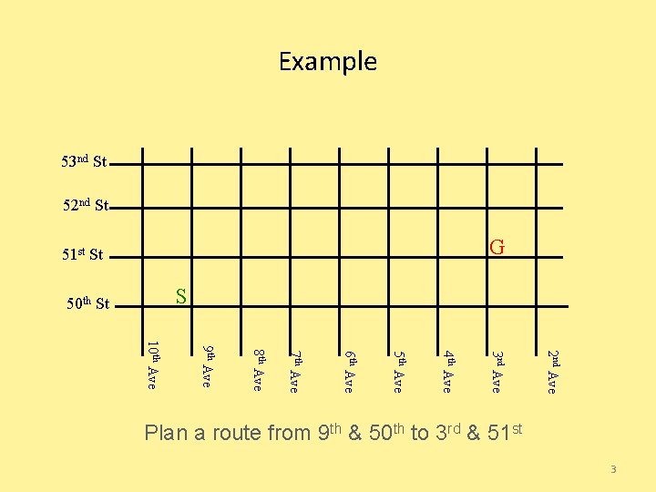
Example 53 nd St 52 nd St G 51 st St S 50 th St 2 nd Ave 3 rd Ave 4 th Ave 5 th Ave 6 th Ave 7 th Ave 8 th Ave 9 th Ave 10 th Ave Plan a route from 9 th & 50 th to 3 rd & 51 st 3

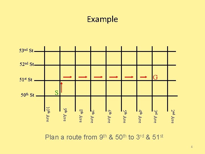
Example 53 nd St 52 nd St G 51 st St S 50 th St 2 nd Ave 3 rd Ave 4 th Ave 5 th Ave 6 th Ave 7 th Ave 8 th Ave 9 th Ave 10 th Ave Plan a route from 9 th & 50 th to 3 rd & 51 st 4

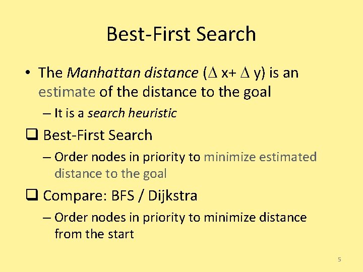
Best-First Search • The Manhattan distance ( x+ y) is an estimate of the distance to the goal – It is a search heuristic q Best-First Search – Order nodes in priority to minimize estimated distance to the goal q Compare: BFS / Dijkstra – Order nodes in priority to minimize distance from the start 5

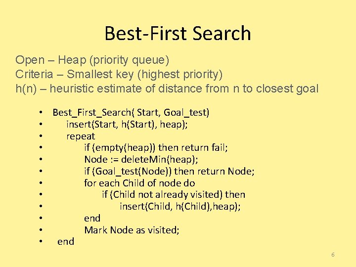
Best-First Search Open – Heap (priority queue) Criteria – Smallest key (highest priority) h(n) – heuristic estimate of distance from n to closest goal • Best_First_Search( Start, Goal_test) • insert(Start, h(Start), heap); • repeat • if (empty(heap)) then return fail; • Node : = delete. Min(heap); • if (Goal_test(Node)) then return Node; • for each Child of node do • if (Child not already visited) then • insert(Child, h(Child), heap); • end • Mark Node as visited; • end 6

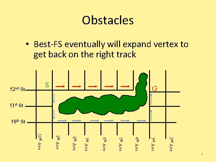
Obstacles • Best-FS eventually will expand vertex to get back on the right track S 52 nd St G 51 st St 50 th St 2 nd Ave 3 rd Ave 4 th Ave 5 th Ave 6 th Ave 7 th Ave 8 th Ave 9 th Ave 10 th Ave 7

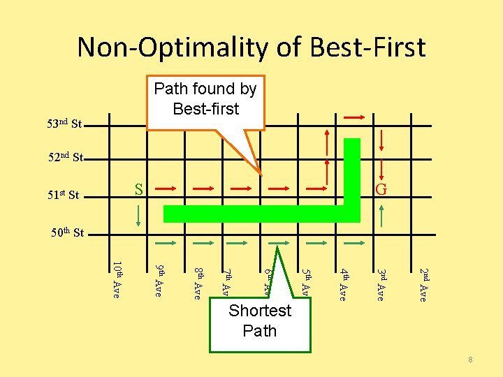
Non-Optimality of Best-First Path found by Best-first 53 nd St 52 nd St S 51 st St G 50 th St 2 nd Ave 3 rd Ave 4 th Ave 5 th Ave 6 th Ave 7 th Ave 8 th Ave 9 th Ave 10 th Ave Shortest Path 8

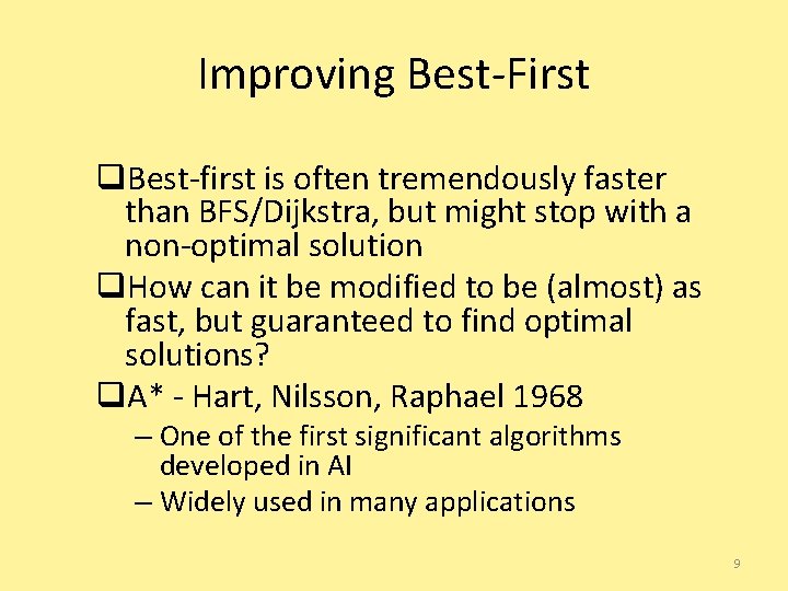
Improving Best-First q. Best-first is often tremendously faster than BFS/Dijkstra, but might stop with a non-optimal solution q. How can it be modified to be (almost) as fast, but guaranteed to find optimal solutions? q. A* - Hart, Nilsson, Raphael 1968 – One of the first significant algorithms developed in AI – Widely used in many applications 9

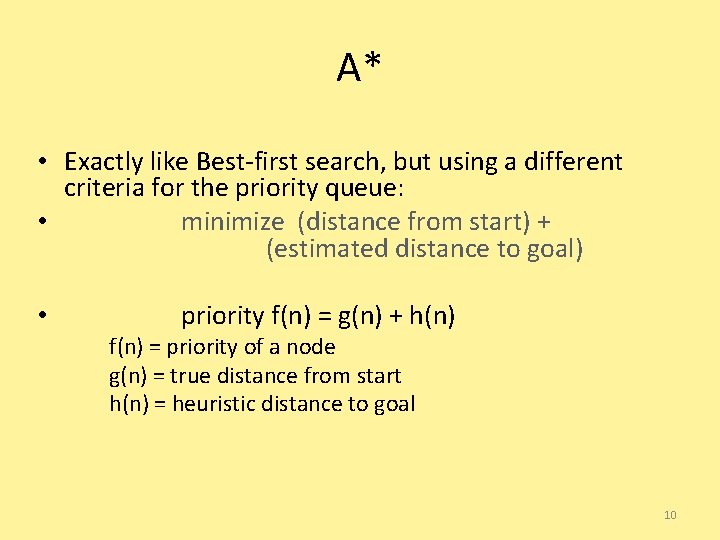
A* • Exactly like Best-first search, but using a different criteria for the priority queue: • minimize (distance from start) + (estimated distance to goal) • priority f(n) = g(n) + h(n) f(n) = priority of a node g(n) = true distance from start h(n) = heuristic distance to goal 10

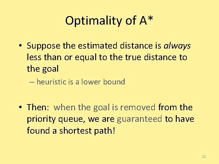
Optimality of A* • Suppose the estimated distance is always less than or equal to the true distance to the goal – heuristic is a lower bound • Then: when the goal is removed from the priority queue, we are guaranteed to have found a shortest path! 11

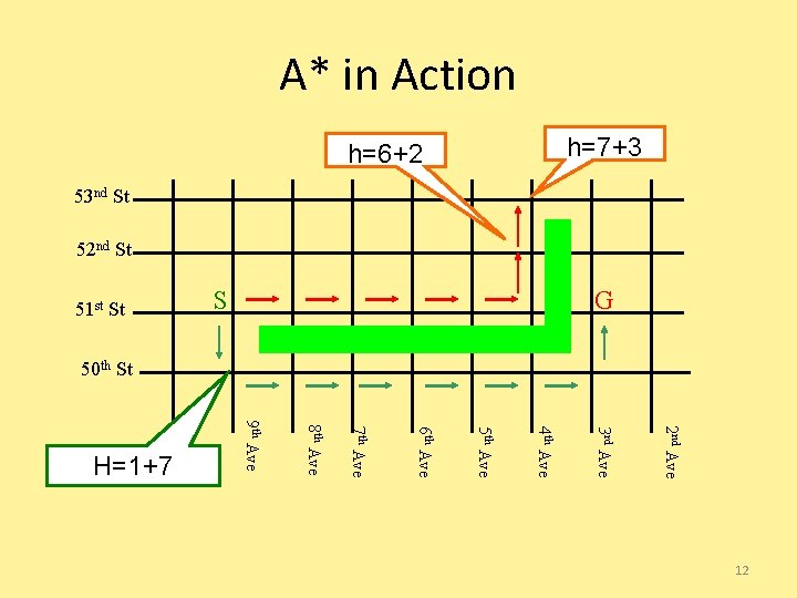
A* in Action 2 nd Ave 3 rd Ave 4 th Ave 5 th Ave 6 th Ave 7 th Ave 8 th Ave 9 th Ave 10 th Ave H=1+7 G S 51 st St h=7+3 h=6+2 53 nd St 52 nd St 50 th St 12

Application of A*: Speech Recognition • (Simplified) Problem: – System hears a sequence of 3 words – It is unsure about what it heard • For each word, it has a set of possible “guesses” • E. g. : Word 1 is one of { “hi”, “high”, “I” } – What is the most likely sentence it heard? 13

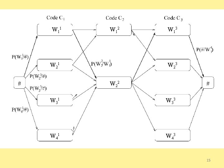
Speech Recognition as Shortest Path • Convert to a shortest-path problem: – Utterance is a “layered” DAG – Begins with a special dummy “start” node – Next: A layer of nodes for each word position, one node for each word choice – Edges between every node in layer i to every node in layer i+1 • Cost of an edge is smaller if the pair of words frequently occur together in real speech – Technically: - log probability of co-occurrence – Finally: a dummy “end” node – Find shortest path from start to end node 14

W 1 1 W 1 2 W 2 1 W 1 3 W 2 2 W W 3111 W 3 3 W 4 1 W 4 3 15

Summary: Graph Search • Depth First – Little memory required – Might find non-optimal path • Breadth First – Much memory required – Always finds optimal path • Iterative Depth-First Search – Repeated depth-first searches, little memory required • Dijskstra’s Short Path Algorithm – Like BFS for weighted graphs • Best First – Can visit fewer nodes – Might find non-optimal path • A* – Can visit fewer nodes than BFS or Dijkstra – Optimal if heuristic estimate is a lower-bound 16

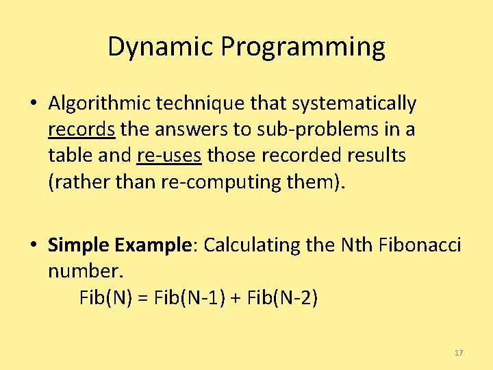
Dynamic Programming • Algorithmic technique that systematically records the answers to sub-problems in a table and re-uses those recorded results (rather than re-computing them). • Simple Example: Calculating the Nth Fibonacci number. Fib(N) = Fib(N-1) + Fib(N-2) 17

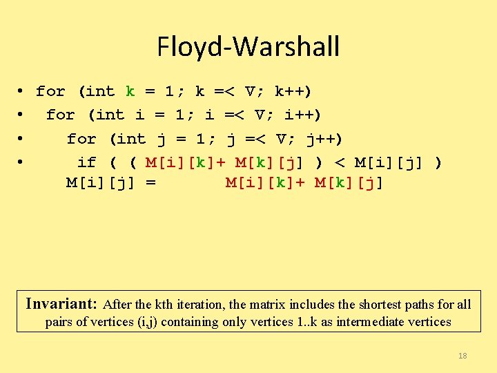
Floyd-Warshall • for (int k = 1; k =< V; k++) • for (int i = 1; i =< V; i++) • for (int j = 1; j =< V; j++) • if ( ( M[i][k]+ M[k][j] ) < M[i][j] ) M[i][j] = M[i][k]+ M[k][j] Invariant: After the kth iteration, the matrix includes the shortest paths for all pairs of vertices (i, j) containing only vertices 1. . k as intermediate vertices 18

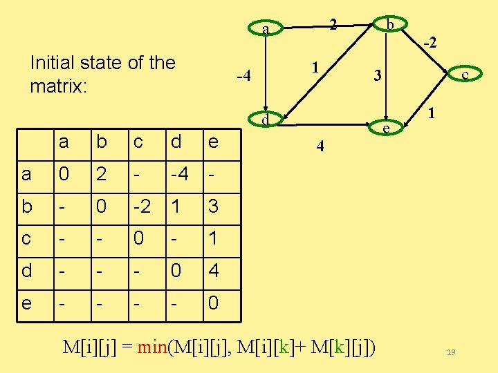
2 a Initial state of the matrix: 1 -4 b b c d e a 0 2 - -4 - b - 0 -2 1 3 c - - 0 - 1 d - - - 0 4 e - - 0 c 3 d a -2 4 M[i][j] = min(M[i][j], M[i][k]+ M[k][j]) e 1 19

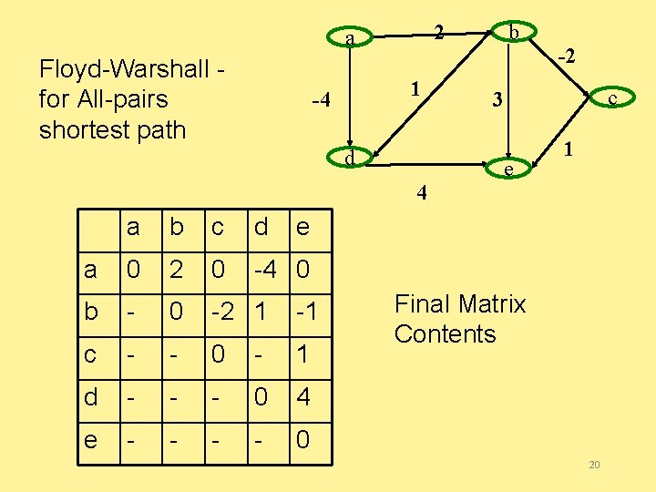
2 a Floyd-Warshall for All-pairs shortest path 1 -4 d 4 a b c d a 0 2 0 -4 0 b - 0 -2 1 -1 c - - 0 - 1 d - - - 0 4 e - - 0 b -2 c 3 e 1 e Final Matrix Contents 20

CSE 326: Data Structures Network Flow 21

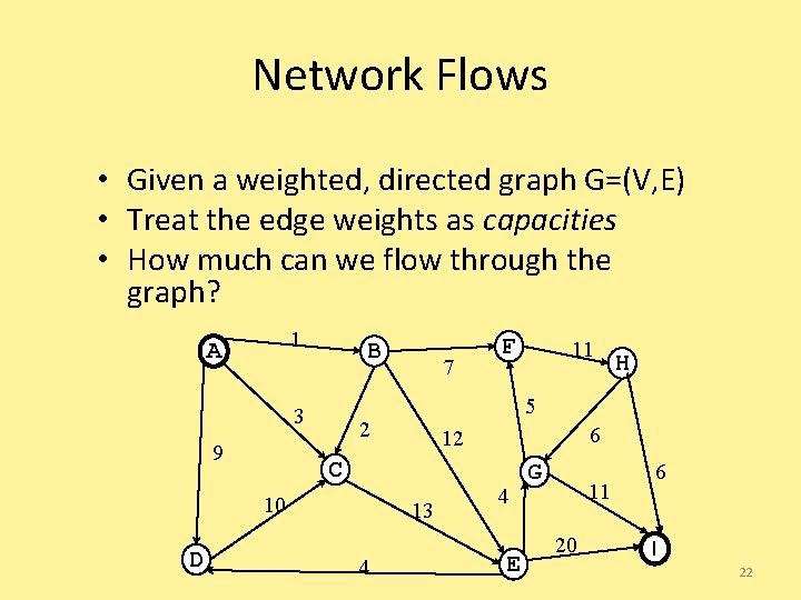
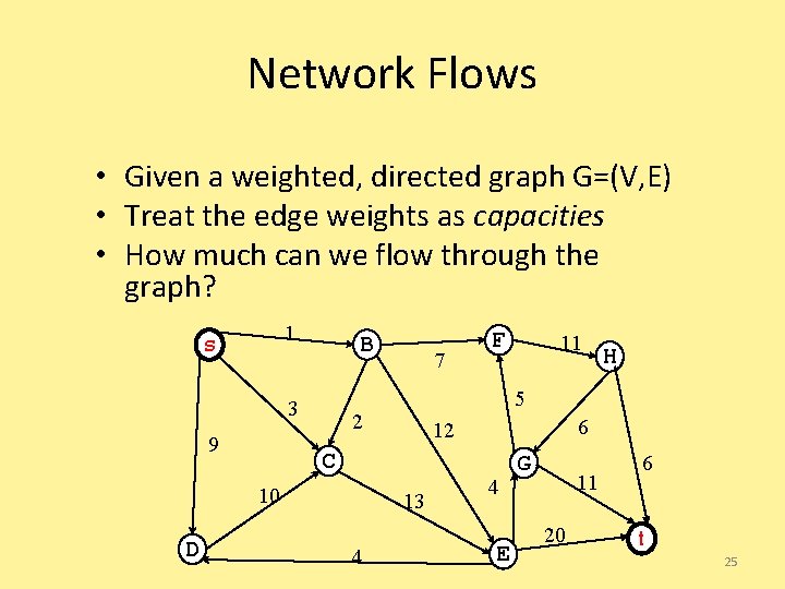
Network Flows • Given a weighted, directed graph G=(V, E) • Treat the edge weights as capacities • How much can we flow through the graph? 1 A B 3 9 H 6 12 C 13 4 11 5 2 10 D 7 F 4 E G 11 20 6 I 22

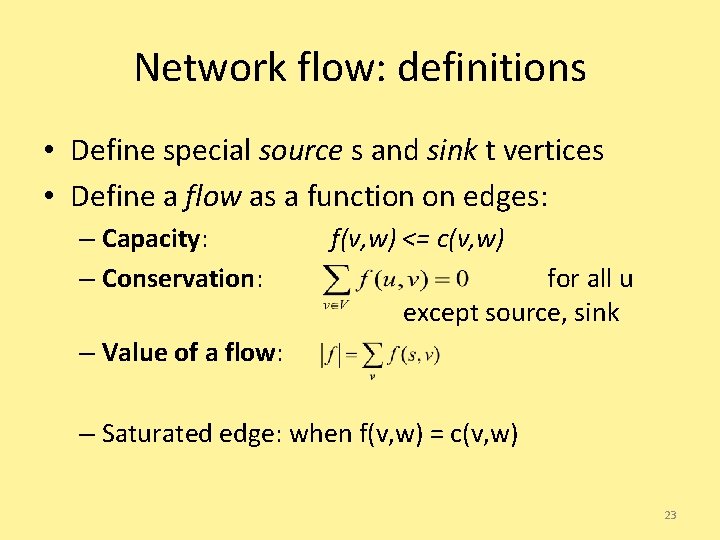
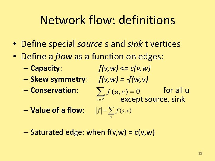
Network flow: definitions • Define special source s and sink t vertices • Define a flow as a function on edges: – Capacity: – Conservation: f(v, w) <= c(v, w) for all u except source, sink – Value of a flow: – Saturated edge: when f(v, w) = c(v, w) 23

Network flow: definitions • Capacity: you can’t overload an edge • Conservation: Flow entering any vertex must equal flow leaving that vertex • We want to maximize the value of a flow, subject to the above constraints 24

Network Flows • Given a weighted, directed graph G=(V, E) • Treat the edge weights as capacities • How much can we flow through the graph? 1 s B 3 9 H 6 12 C 13 4 11 5 2 10 D 7 F 4 E G 11 20 6 t 25

A Good Idea that Doesn’t Work • Start flow at 0 • “While there’s room for more flow, push more flow across the network!” – While there’s some path from s to t, none of whose edges are saturated – Push more flow along the path until some edge is saturated – Called an “augmenting path” 26

How do we know there’s still room? • Construct a residual graph: – Same vertices – Edge weights are the “leftover” capacity on the edges – If there is a path s t at all, then there is still room 27

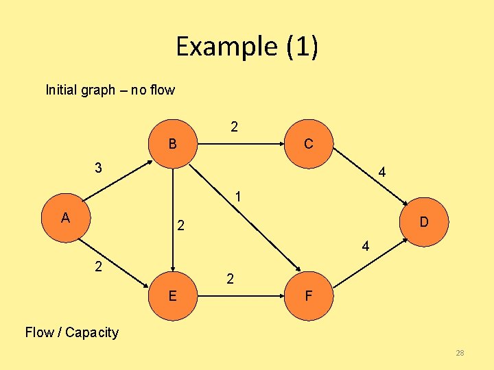
Example (1) Initial graph – no flow 2 B C 3 4 1 A D 2 4 2 2 E F Flow / Capacity 28

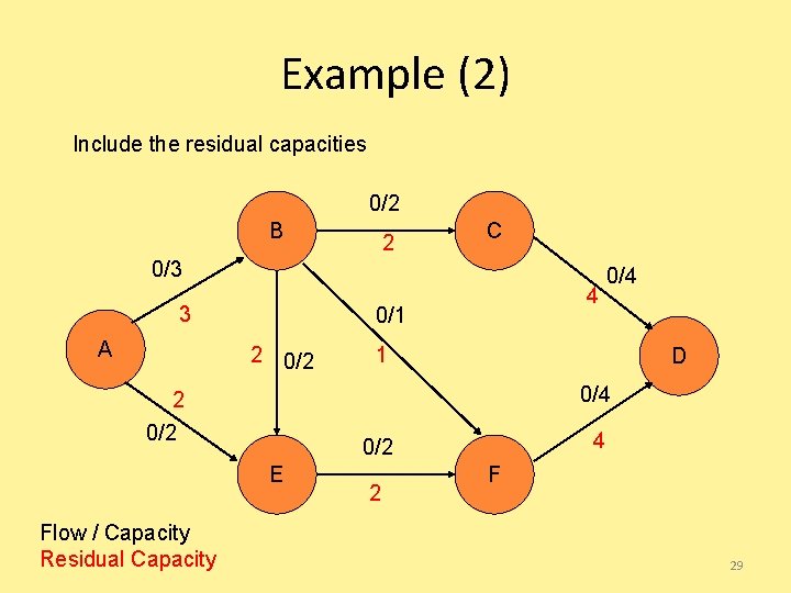
Example (2) Include the residual capacities 0/2 B 2 C 0/3 3 A 0/1 2 0/2 1 D 0/4 2 0/2 4 0/2 E Flow / Capacity Residual Capacity 4 0/4 2 F 29

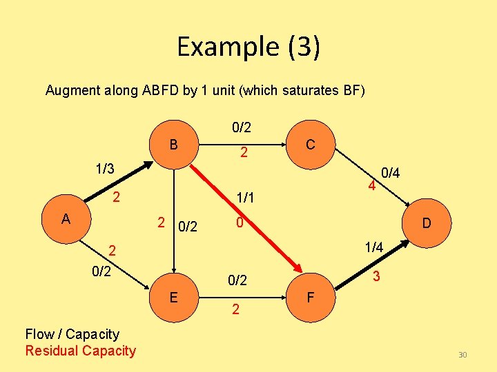
Example (3) Augment along ABFD by 1 unit (which saturates BF) 0/2 B 2 C 1/3 2 A 1/1 2 0/2 0 D 1/4 2 0/2 3 0/2 E Flow / Capacity Residual Capacity 4 0/4 2 F 30

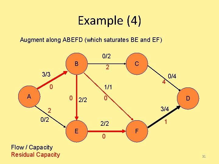
Example (4) Augment along ABEFD (which saturates BE and EF) 0/2 B 2 C 3/3 0 A 1/1 0 2/2 0 D 3/4 2 0/2 1 2/2 E Flow / Capacity Residual Capacity 4 0/4 0 F 31

Now what? • There’s more capacity in the network… • …but there’s no more augmenting paths 32

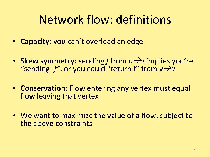
Network flow: definitions • Define special source s and sink t vertices • Define a flow as a function on edges: – Capacity: – Skew symmetry: – Conservation: f(v, w) <= c(v, w) f(v, w) = -f(w, v) for all u except source, sink – Value of a flow: – Saturated edge: when f(v, w) = c(v, w) 33

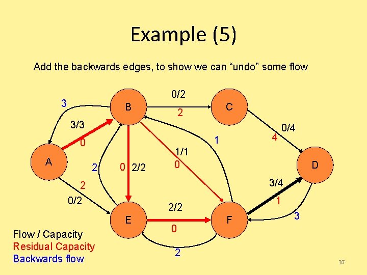
Network flow: definitions • Capacity: you can’t overload an edge • Skew symmetry: sending f from u v implies you’re “sending -f”, or you could “return f” from v u • Conservation: Flow entering any vertex must equal flow leaving that vertex • We want to maximize the value of a flow, subject to the above constraints 34

Main idea: Ford-Fulkerson method • Start flow at 0 • “While there’s room for more flow, push more flow across the network!” – While there’s some path from s to t, none of whose edges are saturated – Push more flow along the path until some edge is saturated – Called an “augmenting path” 35

How do we know there’s still room? • Construct a residual graph: – Same vertices – Edge weights are the “leftover” capacity on the edges – Add extra edges for backwards-capacity too! – If there is a path s t at all, then there is still room 36

Example (5) Add the backwards edges, to show we can “undo” some flow 0/2 3 B C 2 3/3 A 4 1 0 2/2 1/1 0 D 3/4 2 0/2 1 2/2 E Flow / Capacity Residual Capacity Backwards flow 0/4 0 F 3 2 37

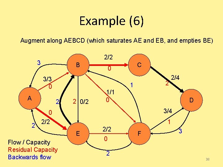
Example (6) Augment along AEBCD (which saturates AE and EB, and empties BE) 2/2 3 B 3/3 0 A 2 C 0 2 1 2 2 0/2 1/1 0 D 3/4 0 2/2 1 E Flow / Capacity Residual Capacity Backwards flow 2/4 2/2 0 F 3 2 38

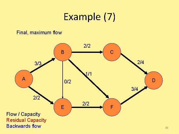
Example (7) Final, maximum flow 2/2 B C 2/4 3/3 1/1 A D 0/2 3/4 2/2 E Flow / Capacity Residual Capacity Backwards flow 2/2 F 39

How should we pick paths? • Two very good heuristics (Edmonds-Karp): – Pick the largest-capacity path available • Otherwise, you’ll just come back to it later…so may as well pick it up now – Pick the shortest augmenting path available • For a good example why… 40

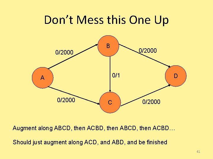
Don’t Mess this One Up 0/2000 B 0/2000 0/1 A 0/2000 C D 0/2000 Augment along ABCD, then ACBD, then ABCD, then ACBD… Should just augment along ACD, and ABD, and be finished 41

Running time? • Each augmenting path can’t get shorter…and it can’t always stay the same length – So we have at most O(E) augmenting paths to compute for each possible length, and there are only O(V) possible lengths. – Each path takes O(E) time to compute • Total time = O(E 2 V) 42

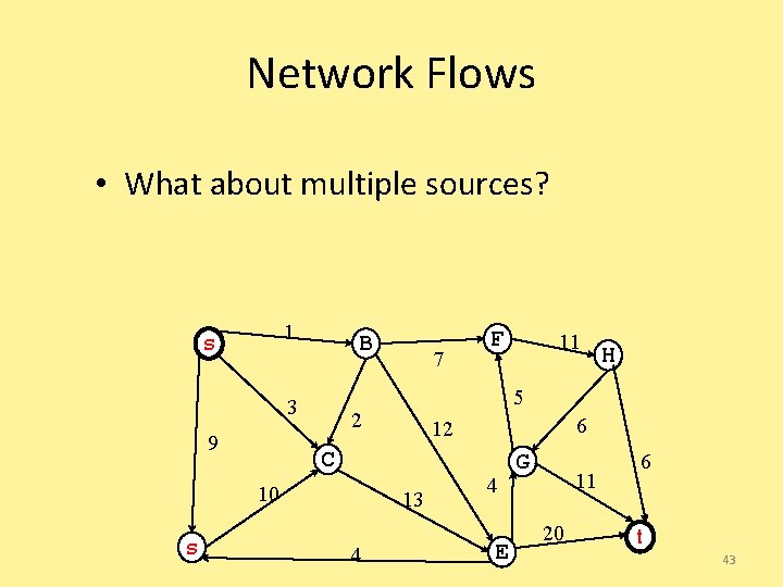
Network Flows • What about multiple sources? 1 s B 3 9 H 6 12 C 13 4 11 5 2 10 s 7 F 4 E G 11 20 6 t 43

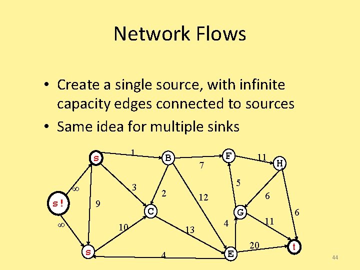
Network Flows • Create a single source, with infinite capacity edges connected to sources • Same idea for multiple sinks 1 s B 3 ∞ s! 9 ∞ H 6 12 C 13 4 11 5 2 10 s 7 F 4 E G 11 20 6 t 44

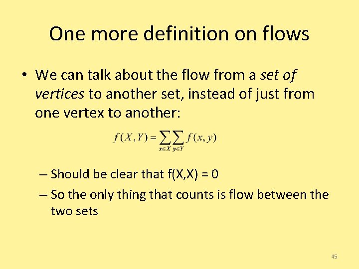
One more definition on flows • We can talk about the flow from a set of vertices to another set, instead of just from one vertex to another: – Should be clear that f(X, X) = 0 – So the only thing that counts is flow between the two sets 45

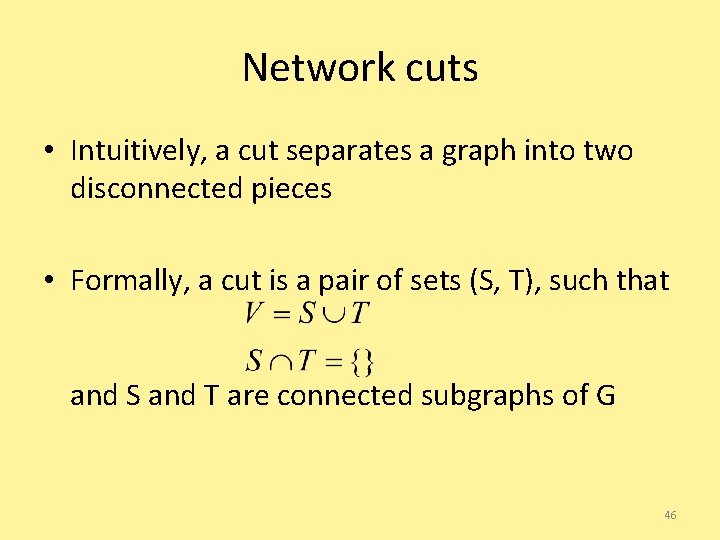
Network cuts • Intuitively, a cut separates a graph into two disconnected pieces • Formally, a cut is a pair of sets (S, T), such that and S and T are connected subgraphs of G 46

Minimum cuts • If we cut G into (S, T), where S contains the source s and T contains the sink t, • Of all the cuts (S, T) we could find, what is the smallest (max) flow f(S, T) we will find? 47

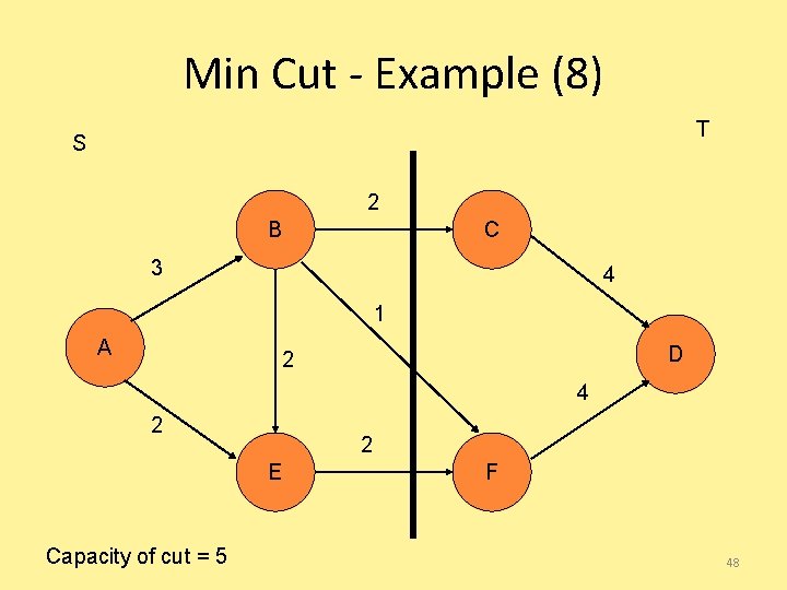
Min Cut - Example (8) T S 2 B C 3 4 1 A D 2 4 2 2 E Capacity of cut = 5 F 48

Coincidence? • NO! Max-flow always equals Min-cut • Why? – If there is a cut with capacity equal to the flow, then we have a maxflow: • We can’t have a flow that’s bigger than the capacity cutting the graph! So any cut puts a bound on the maxflow, and if we have an equality, then we must have a maximum flow. – If we have a maxflow, then there are no augmenting paths left • Or else we could augment the flow along that path, which would yield a higher total flow. – If there are no augmenting paths, we have a cut of capacity equal to the maxflow • Pick a cut (S, T) where S contains all vertices reachable in the residual graph from s, and T is everything else. Then every edge from S to T must be saturated (or else there would be a path in the residual graph). So c(S, T) = f(s, t) = |f| and we’re done. 49

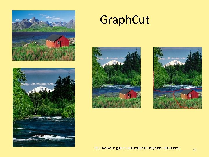
Graph. Cut http: //www. cc. gatech. edu/cpl/projects/graphcuttextures/ 50

CSE 326: Data Structures Dictionaries for Data Compression 51

Dictionary Coding • Does not use statistical knowledge of data. • Encoder: As the input is processed develop a dictionary and transmit the index of strings found in the dictionary. • Decoder: As the code is processed reconstruct the dictionary to invert the process of encoding. • Examples: LZW, LZ 77, Sequitur, • Applications: Unix Compress, gzip, GIF 52

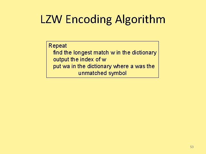
LZW Encoding Algorithm Repeat find the longest match w in the dictionary output the index of w put wa in the dictionary where a was the unmatched symbol 53

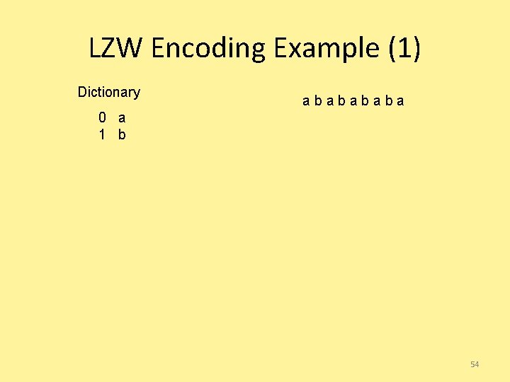
LZW Encoding Example (1) Dictionary ababa 0 a 1 b 54

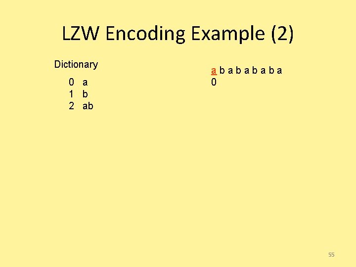
LZW Encoding Example (2) Dictionary 0 a 1 b 2 ab ababa 0 55

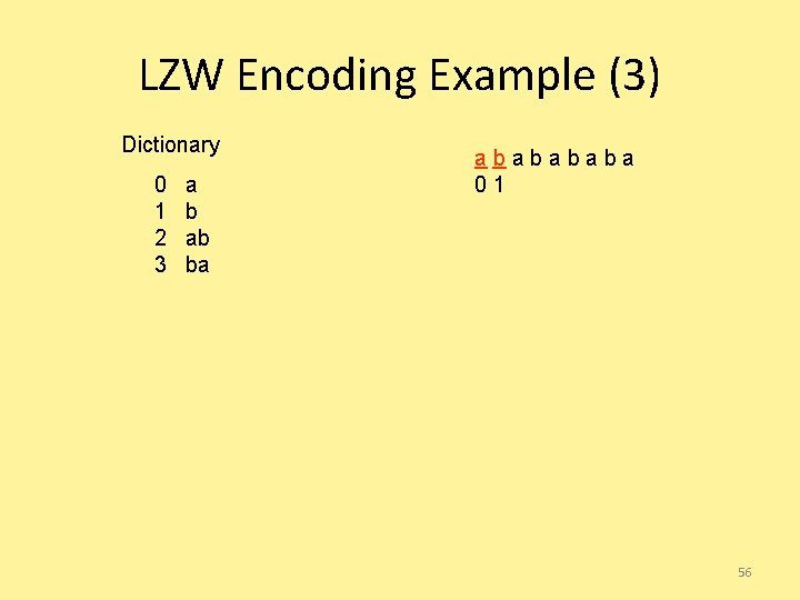
LZW Encoding Example (3) Dictionary 0 1 2 3 a b ab ba ababa 01 56

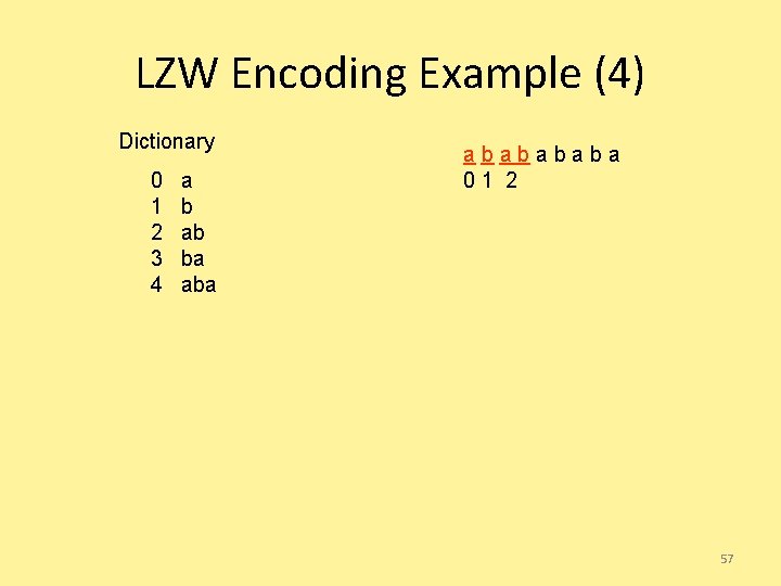
LZW Encoding Example (4) Dictionary 0 1 2 3 4 a b ab ba ababa 01 2 57

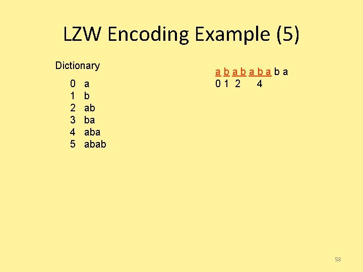
LZW Encoding Example (5) Dictionary 0 1 2 3 4 5 a b ab ba ababa 01 2 4 58

LZW Encoding Example (6) Dictionary 0 1 2 3 4 5 a b ab ba ababa 01 2 4 3 59

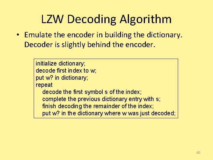
LZW Decoding Algorithm • Emulate the encoder in building the dictionary. Decoder is slightly behind the encoder. initialize dictionary; decode first index to w; put w? in dictionary; repeat decode the first symbol s of the index; complete the previous dictionary entry with s; finish decoding the remainder of the index; put w? in the dictionary where w was just decoded; 60

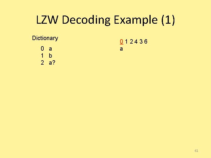
LZW Decoding Example (1) Dictionary 0 a 1 b 2 a? 012436 a 61

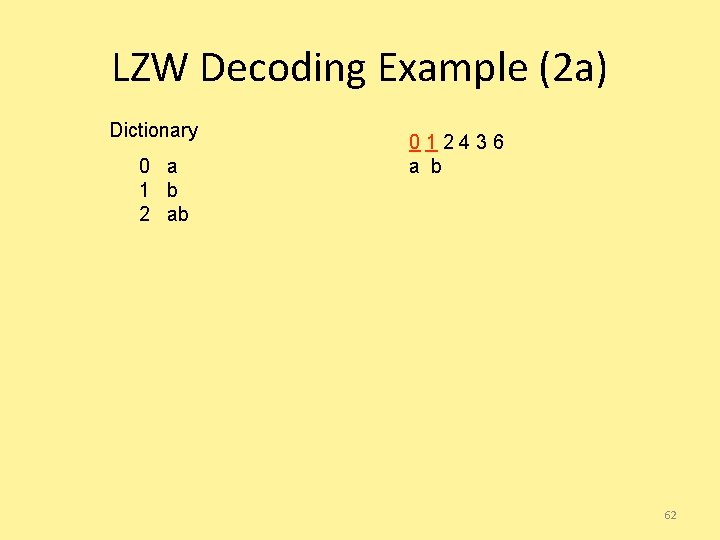
LZW Decoding Example (2 a) Dictionary 0 a 1 b 2 ab 012436 a b 62

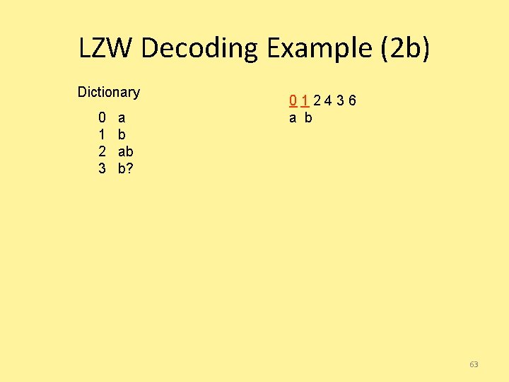
LZW Decoding Example (2 b) Dictionary 0 1 2 3 a b ab b? 012436 a b 63

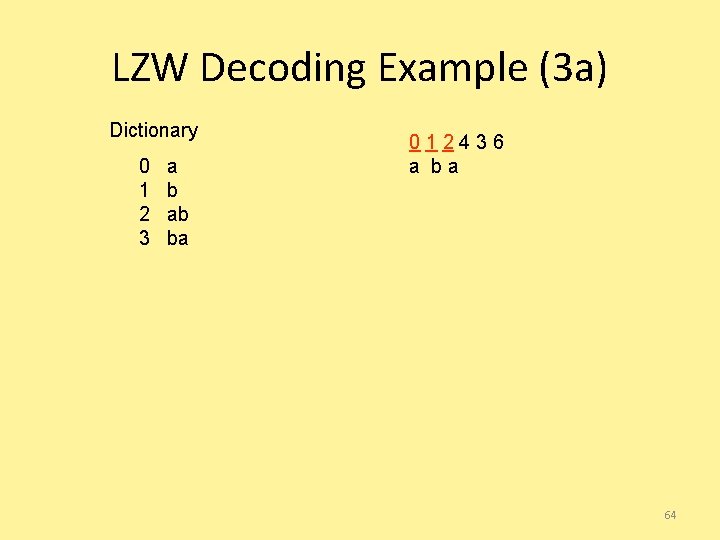
LZW Decoding Example (3 a) Dictionary 0 1 2 3 a b ab ba 012436 a ba 64

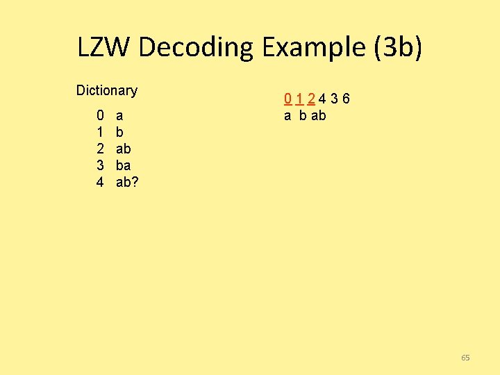
LZW Decoding Example (3 b) Dictionary 0 1 2 3 4 a b ab ba ab? 012436 a b ab 65

LZW Decoding Example (4 a) Dictionary 0 1 2 3 4 a b ab ba aba 012436 a b ab a 66

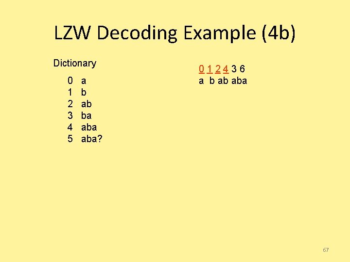
LZW Decoding Example (4 b) Dictionary 0 1 2 3 4 5 a b ab ba aba? 012436 a b ab aba 67

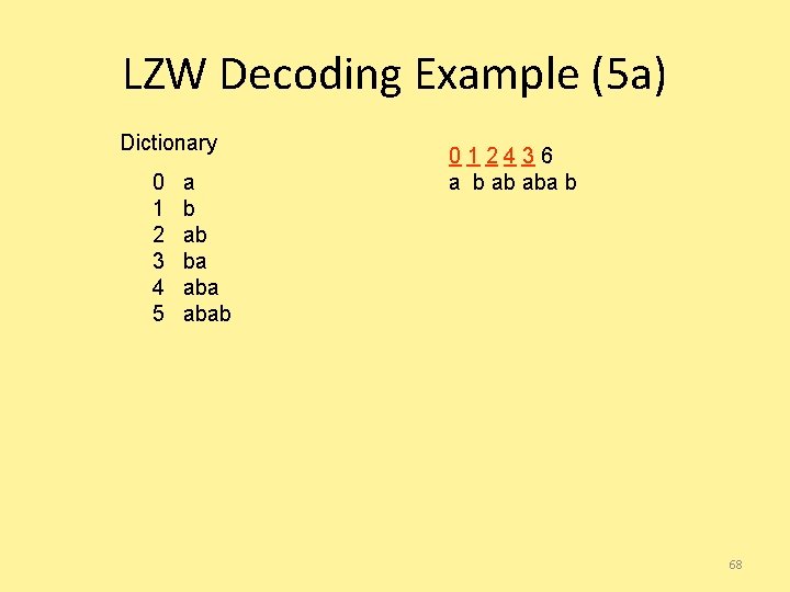
LZW Decoding Example (5 a) Dictionary 0 1 2 3 4 5 a b ab ba abab 012436 a b ab aba b 68

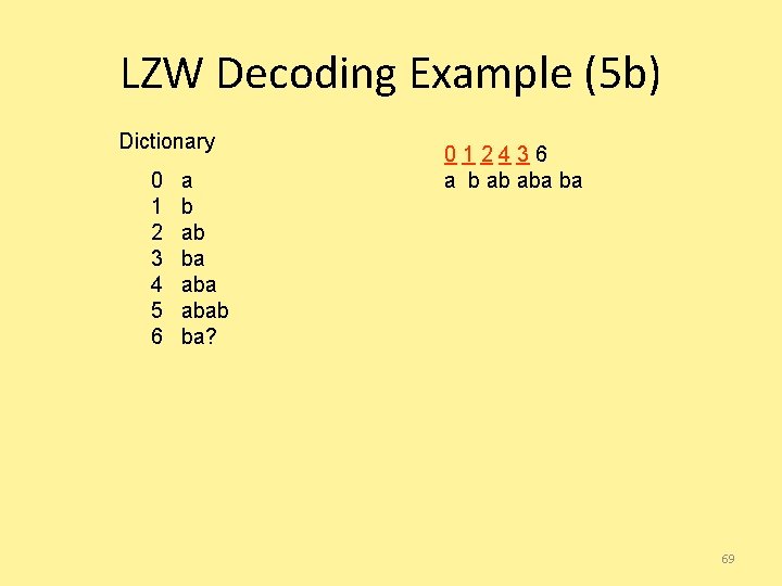
LZW Decoding Example (5 b) Dictionary 0 1 2 3 4 5 6 a b ab ba abab ba? 012436 a b ab aba ba 69

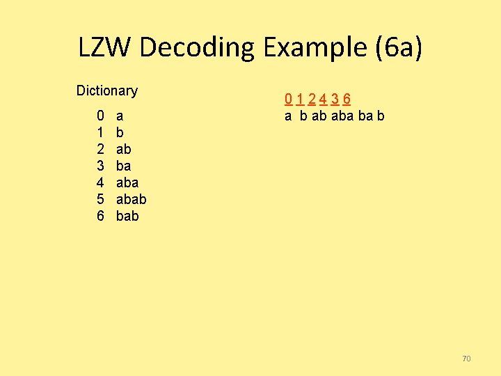
LZW Decoding Example (6 a) Dictionary 0 1 2 3 4 5 6 a b ab ba abab 012436 a b ab aba ba b 70

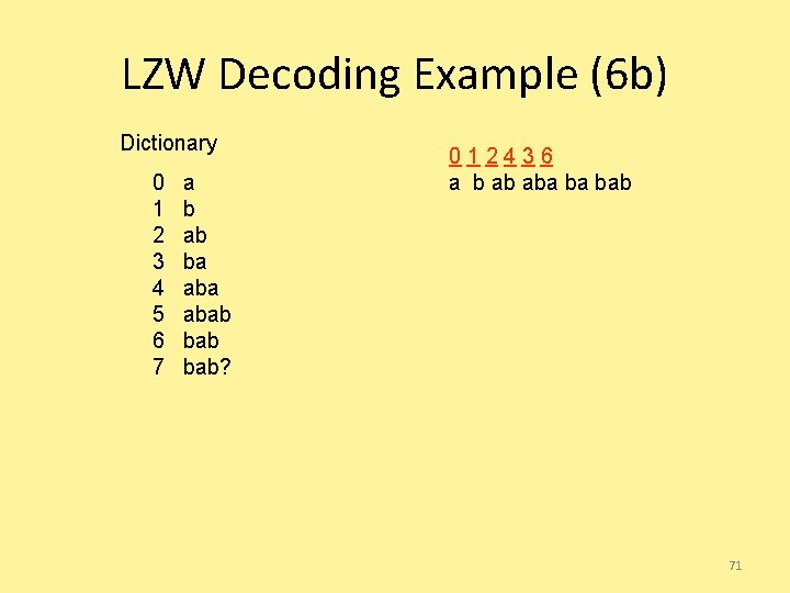
LZW Decoding Example (6 b) Dictionary 0 1 2 3 4 5 6 7 a b ab ba abab bab? 012436 a b ab aba ba bab 71

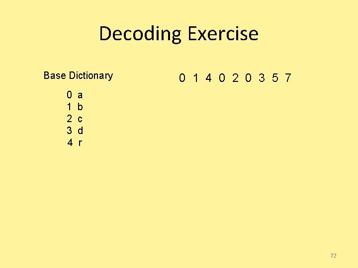
Decoding Exercise Base Dictionary 0 1 2 3 4 0 1 4 0 2 0 3 5 7 a b c d r 72

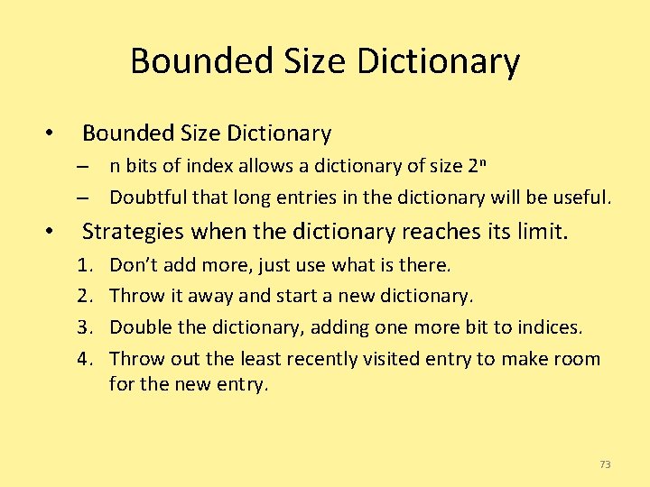
Bounded Size Dictionary • Bounded Size Dictionary – n bits of index allows a dictionary of size 2 n – Doubtful that long entries in the dictionary will be useful. • Strategies when the dictionary reaches its limit. 1. 2. 3. 4. Don’t add more, just use what is there. Throw it away and start a new dictionary. Double the dictionary, adding one more bit to indices. Throw out the least recently visited entry to make room for the new entry. 73

Notes on LZW • Extremely effective when there are repeated patterns in the data that are widely spread. • Negative: Creates entries in the dictionary that may never be used. • Applications: – Unix compress, GIF, V. 42 bis modem standard 74

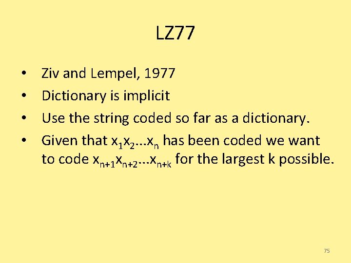
LZ 77 • • Ziv and Lempel, 1977 Dictionary is implicit Use the string coded so far as a dictionary. Given that x 1 x 2. . . xn has been coded we want to code xn+1 xn+2. . . xn+k for the largest k possible. 75

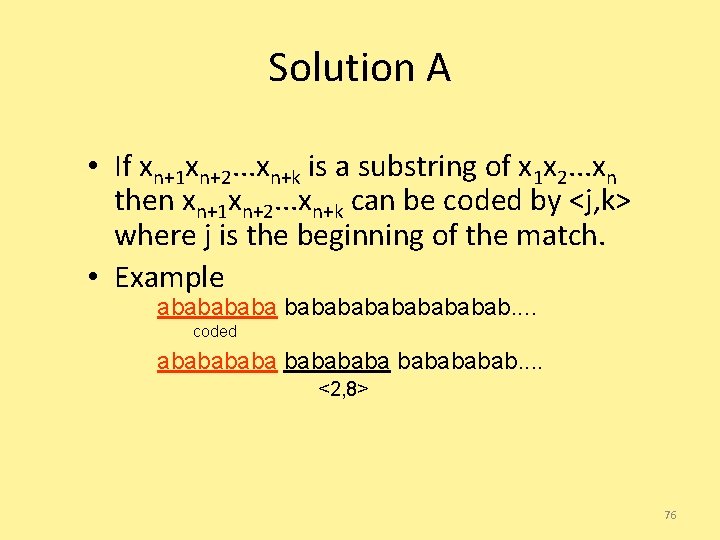
Solution A • If xn+1 xn+2. . . xn+k is a substring of x 1 x 2. . . xn then xn+1 xn+2. . . xn+k can be coded by <j, k> where j is the beginning of the match. • Example ababababab. . coded ababababab. . <2, 8> 76

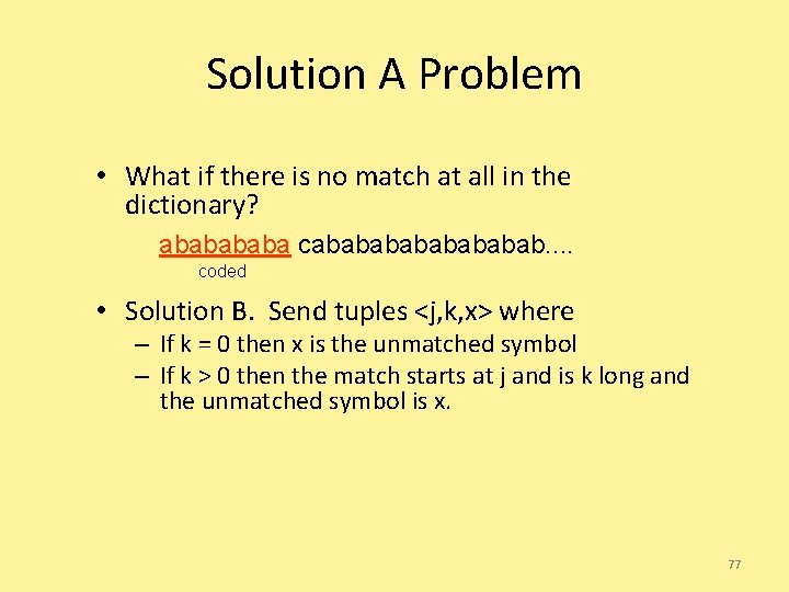
Solution A Problem • What if there is no match at all in the dictionary? ababa cabababab. . coded • Solution B. Send tuples <j, k, x> where – If k = 0 then x is the unmatched symbol – If k > 0 then the match starts at j and is k long and the unmatched symbol is x. 77

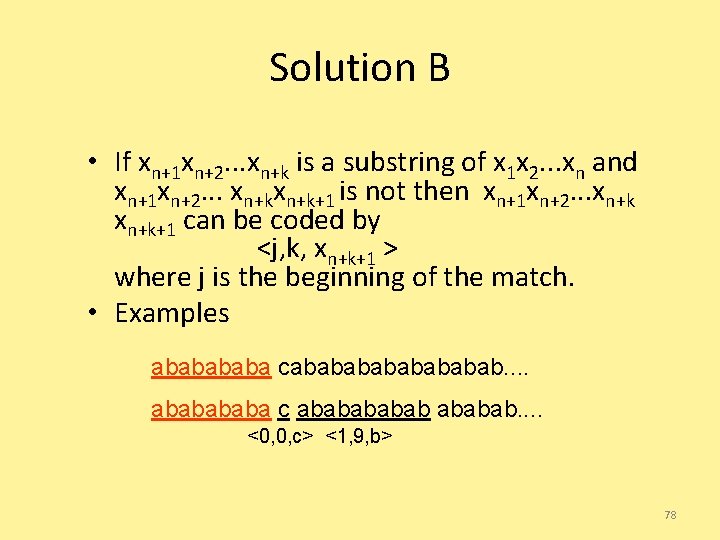
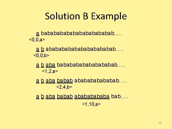
Solution B • If xn+1 xn+2. . . xn+k is a substring of x 1 x 2. . . xn and xn+1 xn+2. . . xn+k+1 is not then xn+1 xn+2. . . xn+k+1 can be coded by <j, k, xn+k+1 > where j is the beginning of the match. • Examples ababa cabababab. . ababa c ababab. . <0, 0, c> <1, 9, b> 78

Solution B Example a babababababab. . . <0, 0, a> a b abababababab. . . <0, 0, b> a b aba bababababab. . . <1, 2, a> a b aba babababab. . . <2, 4, b> a b aba babababa bab. . . <1, 10, a> 79

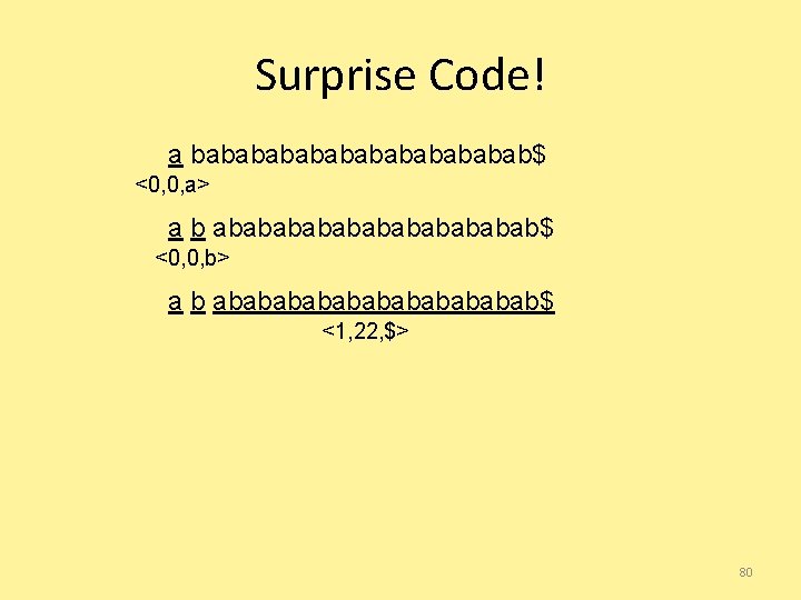
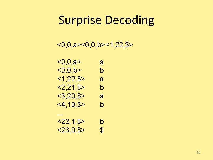
Surprise Code! a babababababab$ <0, 0, a> a b abababababab$ <0, 0, b> a b abababababab$ <1, 22, $> 80

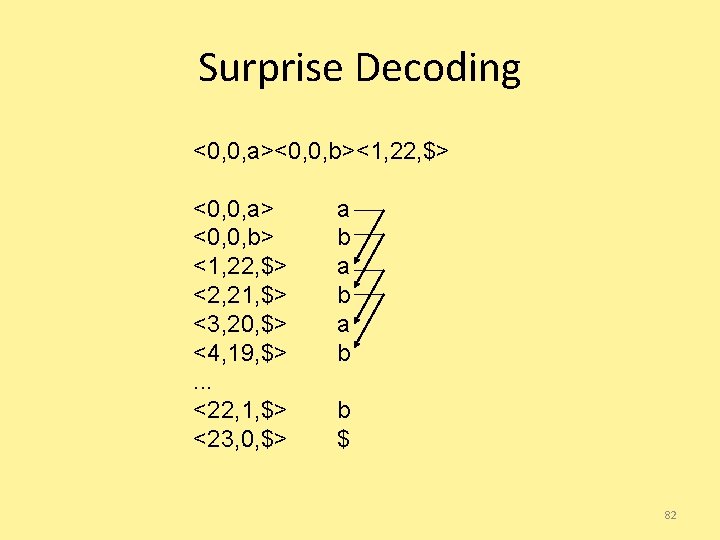
Surprise Decoding <0, 0, a><0, 0, b><1, 22, $> <0, 0, a> <0, 0, b> <1, 22, $> <2, 21, $> <3, 20, $> <4, 19, $>. . . <22, 1, $> <23, 0, $> a b a b b $ 81

Surprise Decoding <0, 0, a><0, 0, b><1, 22, $> <0, 0, a> <0, 0, b> <1, 22, $> <2, 21, $> <3, 20, $> <4, 19, $>. . . <22, 1, $> <23, 0, $> a b a b b $ 82

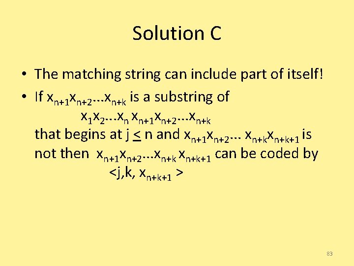
Solution C • The matching string can include part of itself! • If xn+1 xn+2. . . xn+k is a substring of x 1 x 2. . . xn xn+1 xn+2. . . xn+k that begins at j < n and xn+1 xn+2. . . xn+k+1 is not then xn+1 xn+2. . . xn+k+1 can be coded by <j, k, xn+k+1 > 83

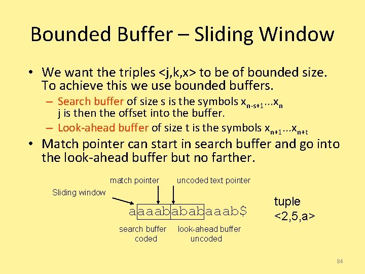
Bounded Buffer – Sliding Window • We want the triples <j, k, x> to be of bounded size. To achieve this we use bounded buffers. – Search buffer of size s is the symbols xn-s+1. . . xn j is then the offset into the buffer. – Look-ahead buffer of size t is the symbols xn+1. . . xn+t • Match pointer can start in search buffer and go into the look-ahead buffer but no farther. match pointer uncoded text pointer Sliding window aaaabababaaab$ search buffer coded tuple <2, 5, a> look-ahead buffer uncoded 84