Chapter 4 Informed Search Uninformed searches easy l

Chapter 4 Informed Search Uninformed searches easy l but very inefficient in most cases l of huge search tree l Informed searches uses problem-specific information l to reduce the search tree into a small one l l resolve time and memory complexities

Informed (Heuristic) Search Best-first search l It uses an evaluation function, f(n) l l to determine the desirability of expanding nodes, making an order The order of expanding nodes is essential to the size of the search tree l less space, faster l

Best-first search Every node is then l attached with a value stating its goodness The nodes in the queue arranged l in the order that the best one is placed first However this order doesn't guarantee l the node to expand is really the best The node only appears to be best l because, in reality, the evaluation is not omniscient (全 能)

Best-first search The path cost g is one of the example l However, it doesn't direct the search toward the goal Heuristic (聰明) function h(n) is required l Estimate cost of the cheapest path l l Expand the node closest to the goal l l from node n to a goal state = Expand the node with least cost If n is a goal state, h(n) = 0

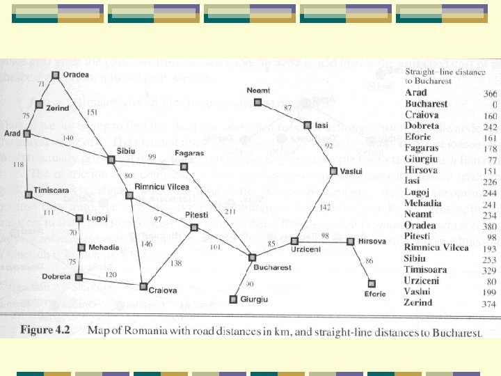
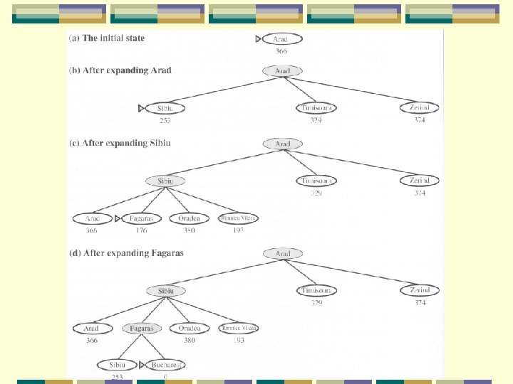
Greedy best-first search Tries to expand the node closest to the goal l because it’s likely to lead to a solution quickly l Just evaluates the node n by l heuristic function: f(n) = h(n) E. g. , SLD – Straight Line Distance l h. SLD

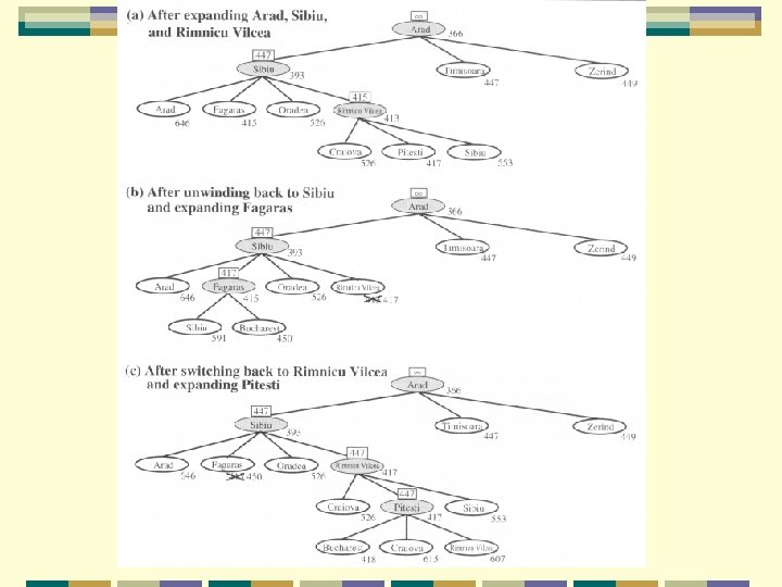
Greedy best-first search Goal is Bucharest Initial state is Arad h. SLD cannot be computed from the problem itself l only obtainable from some amount of experience l

Greedy best-first search It is good ideally but poor practically l since we cannot make sure a heuristic is good l Also, it just depends on estimates on future cost

Analysis of greedy search Similar to depth-first search not optimal l incomplete l suffers from the problem of repeated states l l l causing the solution never be found The time and space complexities l depends on the quality of h

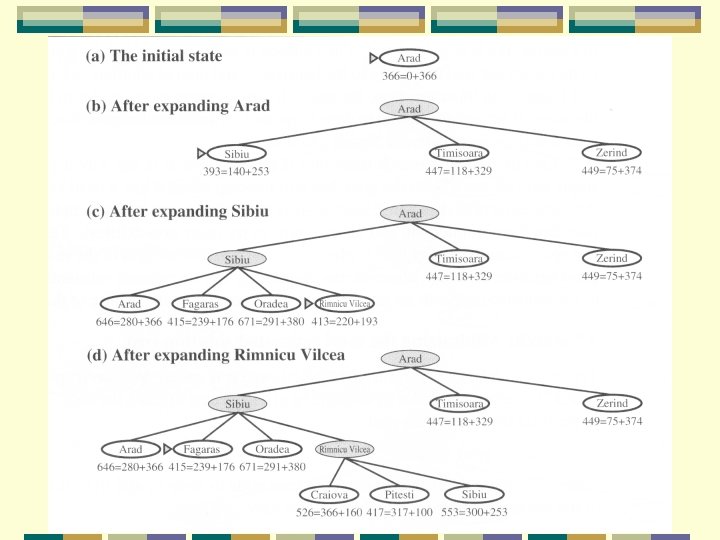
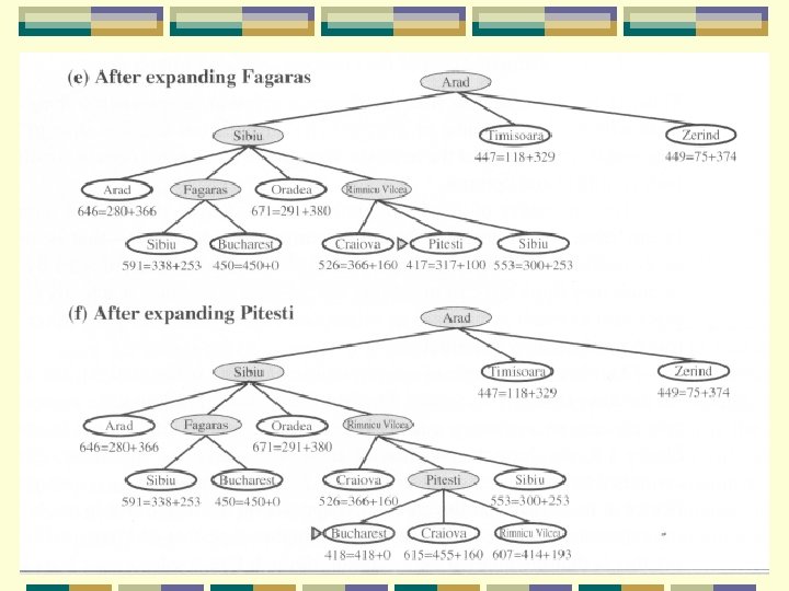
A* search The most well-known best-first search l evaluates nodes by combining path cost g(n) and heuristic h(n) l f(n) = g(n) + h(n) l g(n) – cheapest known path l f(n) – cheapest estimated path l Minimizing the total path cost by combining uniform-cost search l and greedy search l

A* search Uniform-cost search optimal and complete l minimizes the cost of the path so far, g(n) l but can be very inefficient l greedy search + uniform-cost search evaluation function is f(n) = g(n) + h(n) l [evaluated so far + estimated future] l f(n) = estimated cost of the cheapest solution through n l

Analysis of A* search is complete and optimal l time and space complexities are reasonable l But optimality can only be assured when h(n) is admissible l h(n) never overestimates the cost to reach the goal l we can underestimate h. SLD, overestimate?

Memory bounded search Memory another issue besides the time constraint l even more important than time l because a solution cannot be found l if not enough memory is available l l A solution can still be found l even though a long time is needed

Iterative deepening A* search IDA* = Iterative deepening (ID) + A* l As ID effectively reduces memory constraints l complete l and optimal l because it is indeed A* IDA* uses f-cost(g+h) for cutoff rather than depth l the cutoff value is the smallest f-cost of any node l l that exceeded the cutoff value on the previous iteration

RBFS Recursive best-first search similar to depth-first search l which goes recursively in depth l except RBFS keeps track of f-value l It remembers the best f-value in the forgotten subtrees l if necessary, re-expand the nodes l

RBFS optimal if h(n) is admissible l space complexity is: O(bd) l IDA* and RBFS suffer from using too little memory l just keep track of f-cost and some information l Even if more memory were available, l IDA* and RBFS cannot make use of them

Simplified memory A* search Weakness of IDA* and RBFS only keeps a simple number: f-cost limit l This may be trapped by repeated states l IDA* is modified to SMA* the current path is checked for repeated states l but unable to avoid repeated states generated by alternative paths l SMA* uses a history of nodes to avoid repeated states

Simplified memory A* search SMA* has the following properties: utilize whatever memory is made available to it l avoids repeated states as far as its memory allows, by deletion l complete if the available memory l l l is sufficient to store the shallowest solution path optimal if enough memory l is available to store the shallowest optimal solution path

Simplified memory A* search l Otherwise, it returns the best solution that l l can be reached with the available memory When enough memory is available for the entire search tree l the search is optimally efficient When SMA* has no memory left l it drops a node from the queue (tree) that is unpromising (seems to fail)

Simplified memory A* search To avoid re-exploring, similar to RBFS, l it keeps information in the ancestor nodes l about quality of the best path in the forgotten subtree If all other paths have been shown to be worse than the path it has forgotten l it regenerates the forgotten subtree l SMA* can solve more difficult problems than A* (larger tree)

Simplified memory A* search However, SMA* has to l repeatedly regenerate the same nodes for some problem The problem becomes intractable (難解決 ) for SMA* even though it would be tractable (可解決) for A*, with unlimited memory l (it takes too long time!!!) l

Simplified memory A* search Trade-off should be made l but unfortunately there is no guideline for this inescapable problem The only way drops the optimality requirement at this situation l Once a solution is found, return & finish. l

Heuristic functions For the problem of 8 -puzzle l two heuristic functions can be applied l to cut down the search tree h 1 = the number of misplaced tiles l h 1 is admissible because it never overestimates l l at least h 1 steps to reach the goal.

Heuristic functions h 2= the sum of distances of the tiles from their goal positions l This distance is called city block distance or Manhattan distance l l l as it counts horizontally and vertically h 2 is also admissible, in the example: h 2 = 3 + 1 + 2 + 2 + 3 + 2 = 18 l True cost = 26 l

The effect of heuristic accuracy on performance effective branching factor b* can represent the quality of a heuristic l N = the total number of nodes expanded by A* l the solution depth is d l and b* is the branching factor of the uniform tree l l l N = 1 + b* + (b*)2 + …. + (b*)d N is small if b* tends to 1

The effect of heuristic accuracy on performance h 2 dominates h 1 if for any node, h 2(n) ≥ h 1(n) Conclusion: l always better to use a heuristic function with higher values, as long as it does not overestimate

The effect of heuristic accuracy on performance

Inventing admissible heuristic functions relaxed problem l A problem with less restriction on the operators It is often the case that l the cost of an exact solution to a relaxed problem l is a good heuristic for the original problem

Inventing admissible heuristic functions Original problem: l A tile can move from square A to square B l l if A is horizontally or vertically adjacent to B and B is blank Relaxed problem: 1. A tile can move from square A to square B l 2. A tile can move from square A to square B l 3. if A is horizontally or vertically adjacent to B if B is blank A tile can move from square A to square B

Inventing admissible heuristic functions If one doesn't know the “clearly best” heuristic among the h 1, …, hm heuristics l then set h(n) = max(h 1(n), …, hm(n)) l i. e. , let the computer run it l l Determine at run time

Inventing admissible heuristic functions Admissible heuristic can also be derived from the solution cost l of a subproblem of a given problem l getting only 4 tiles into their positions l cost of the optimal solution of this subproblem l l used as a lower bound

Local search algorithms So far, we are finding solution paths by searching (Initial state goal state) In many problems, however, l l l the path to goal is irrelevant to solution e. g. , 8 -queens problem solution l l the final configuration not the order they are added or modified Hence we can consider other kinds of method l Local search

Local search Just operate on a single current state l rather than multiple paths Generally move only to l neighbors of that state The paths followed by the search are not retained l hence the method is not systematic l

Local search Two advantages of l uses little memory – a constant amount l l for current state and some information can find reasonable solutions in large or infinite (continuous) state spaces l where systematic algorithms are unsuitable l Also suitable for optimization problems l finding the best state according to l l an objective function

Local search State space landscape has two axis location (defined by states) l elevation (defined by objective function) l

Local search A complete local search algorithm l always finds a goal if one exists An optimal algorithm l always finds a global maximum/minimum

Hill-climbing search simply a loop It continually moves in the direction of increasing value l i. e. , uphill l No search tree is maintained The node need only record the state l its evaluation (value, real number) l

Hill-climbing search Evaluation function calculates the cost l a quantity instead of a quality l When there is more than one best successor to choose from l the algorithm can select among them at random

Hill-climbing search

Drawbacks of Hill-climbing search Hill-climbing is also called greedy local search l grabs a good neighbor state l l without thinking about where to go next. Local maxima: The peaks lower than the highest peak in the state space l The algorithm stops even though the solution is far from satisfactory l

Drawbacks of Hill-climbing search Ridges (山脊) The grid of states is overlapped on a ridge rising from left to right l Unless there happen to be operators l moving directly along the top of the ridge l the search may oscillate from side to side, making little progress l

Drawbacks of Hill-climbing search Plateaux: (平原) l an area of the state space landscape where the evaluation function is flat l shoulder l impossible to make progress l l Hill-climbing might be unable to l find its way off the plateau

Solution Random-restart hill-climbing resolves these problems l It conducts a series of hill-climbing searches from random generated initial states l the best result found so far is saved from any of the searches l It can use a fixed number of iterations l Continue until the best saved result has not been improved l l for a certain number of iterations

Solution Optimality cannot be ensured However, a reasonably good solution can usually be found

Simulated annealing Instead of starting again randomly l the search can take some downhill steps to leave the local maximum l Annealing is the process of gradually cooling a liquid until it freezes l allowing the downhill steps l

Simulated annealing The best move is not chosen l instead a random one is chosen If the move actually results better it is always executed l Otherwise, the algorithm takes the move with a probability less than 1 l

Simulated annealing

Simulated annealing The probability decreases exponentially with the “badness” of the move l = ΔE l T also affects the probability SinceΔE 0, T > 0 l the probability is taken as 0 < eΔE/T 1

Simulated annealing The higher T is the more likely the bad move is allowed l When T is large and ΔE is small ( 0) l l ΔE/T is a negative small value eΔE/T is close to 1 T becomes smaller and smaller until T = 0 At that time, SA becomes a normal hill-climbing l The schedule determines the rate at which T is lowered l

Local beam search Keeping only one current state is no good Hence local beam search keeps k states l all k states are randomly generated initially l at each step, l l all successors of k states are generated If any one is a goal, then halt!! l else select the k best successors l l from the complete list and repeat

Local beam search different from random-restart hill-climbing l RRHC makes k independent searches Local beam search will work together collaboration l choosing the best successors l l among those generated together by the k states Stochastic beam search choose k successors at random l rather than k best successors l

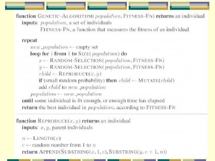
Genetic Algorithms GA a variant of stochastic beam search l successor states are generated by l combining two parent states l rather than modifying a single state l l successor state is called an “offspring” GA works by first making a population l a set of k randomly generated states l

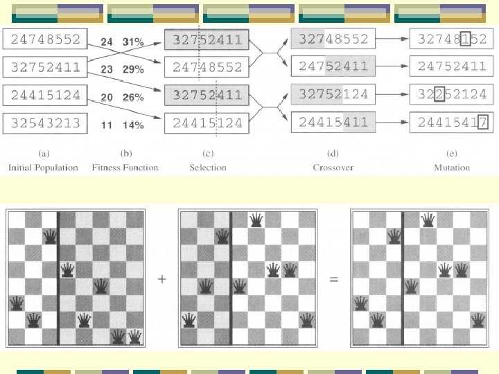
Genetic Algorithms Each state, or individual l represented as a string over a finite alphabet, e. g. , binary or 1 to 8, etc. The production of next generation of states is rated by the evaluation function l or fitness function l l returns higher values for better states Next generation is chosen l based on some probabilities fitness function

Genetic Algorithms Operations for reproduction l cross-over combining two parent states randomly l cross-over point is randomly chosen from the positions in the string l l mutation l modifying the state randomly with a small independent probability Efficiency and effectiveness are based on the state representation l different algorithms l

In continuous spaces Finding out the optimal solutions using steepest gradient method l partial derivatives l Suppose we have a function of 6 variables The gradient of f is then l giving the magnitude and direction of the steepest slope

In continuous spaces By setting l we can find a maximum or minimum However, this value is just a local optimum l not a global optimum l We can still perform steepest-ascent hillclimbing via to gradually find the global solution l α is a small constant, defined by user l

Online search agents So far, all algorithms are offline l a solution is computed before acting However, it is sometimes impossible hence interleaving is necessary l compute, act, computer, act, … l this is suitable l for dynamic or semidynamic environment l exploration problem with unknown states and actions l

Online local search Hill-climbing search just keeps one current state in memory l generate a new state to see its goodness l it is already an online search algorithm l but unfortunately not very useful l because of local maxima and cannot leave off l l random-restart is also useless l l the agent cannot restart again then random walk is used

Random walk simply selects at random one of the available actions from the current state l preference can be given to actions l l that have not yet been tried If the space is finite random walk will eventually find a goal l but the process can be very slow l