Local Search Algorithms Local Search Combinatorial problems involve

Local Search Algorithms

Local Search

Combinatorial problems. . . • involve finding a grouping, ordering, or assignment of a discrete set of objects which satisfies certain constraints • arise in many domains of computer science and various application areas • have high computational complexity (NPhard) • are solved in practice by searching an exponentially large space of candidate / partial solutions

Examples for combinatorial problems: • finding shortest/cheapest round trips (TSP) • finding models of propositional formulae (SAT) • planning, scheduling, time-tabling • resource allocation • protein structure prediction • genome sequence assembly

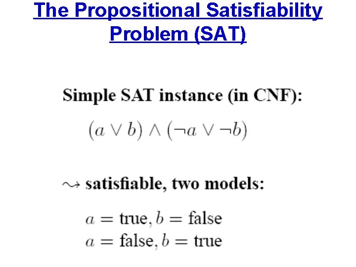
The Propositional Satisfiability Problem (SAT)

SAT

The Traveling Salesperson Problem (TSP) • TSP – optimization variant: • For a given weighted graph G = (V, E, w), find a Hamiltonian cycle in G with minimal weight, • i. e. , find the shortest round-trip visiting each vertex exactly once. • TSP – decision variant: • For a given weighted graph G = (V, E, w), decide whether a Hamiltonian cycle with minimal weight ≤ b exists in G.

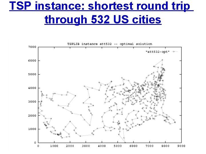
TSP instance: shortest round trip through 532 US cities

Search Methods • • Types of search methods: systematic ←→ local search deterministic ←→ stochastic sequential ←→ parallel

Local Search (LS) Algorithms • search space S (SAT: set of all complete truth assignments to propositional variables) • solution set (SAT: models of given formula) • neighborhood relation (SAT: neighboring variable assignments differ in the truth value of exactly one variable) • evaluation function g : S → R+ (SAT: number of clauses unsatisfied under given assignment)

Local Search: • start from initial position • iteratively move from current position to neighboring position • use evaluation function for guidance Two main classes: • local search on partial solutions • local search on complete solutions

local search on partial solutions

Local search for partial solutions • Order the variables in some order. • Span a tree such that at each level a given value is assigned a value. • Perform a depth-first search. • But, use heuristics to guide the search. Choose the best child according to some heuristics. (DFS with node ordering)

Construction Heuristics for partial solutions • search space: space of partial solutions • search steps: extend partial solutions with assignment for the next element • solution elements are often ranked according to a greedy evaluation function

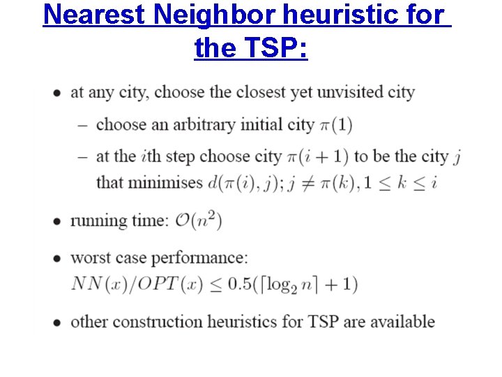
Nearest Neighbor heuristic for the TSP:

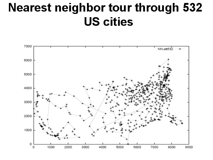
Nearest neighbor tour through 532 US cities

DFS • Once a solution has been found (with the first dive into the tree) we can continue search the tree with DFS and backtracking. • In fact, this is what we did with DFBn. B. • DFBn. B with node ordering.

Limited Discrepancy Search • At each node, the heuristic prefers one of the children. • A discrepancy is when you go against the heuristic. • Perform DFS from the root node with k discrepancies • Start with k=0 • Then increasing k by 1 • Stop at anytime.

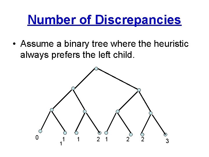
Number of Discrepancies • Assume a binary tree where the heuristic always prefers the left child. 0 1 1 1 2 2 3

Limited Discrepancy Search Advantages: • Anytime algorithm • Solutions are ordered according to heuristics

local search on complete solutions

Iterative Improvement (Greedy Search): • initialize search at some point of search space • in each step, move from the current search position to a neighboring position with better evaluation function value

Iterative Improvement for SAT • initialization: randomly chosen, complete truth assignment • neighborhood: variable assignments are neighbors iff they differ in truth value of one variable • neighborhood size: O(n) where n = number of variables • evaluation function: number of clauses unsatisfied under given assignment

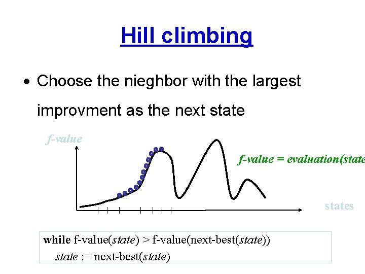
Hill climbing · Choose the nieghbor with the largest improvment as the next state f-value = evaluation(states while f-value(state) > f-value(next-best(state)) state : = next-best(state)

Hill climbing function Hill-Climbing(problem) returns a solution state current Make-Node(Initial-State[problem]) loop do next a highest-valued successor of current if Value[next] < Value[current] then return current next end

Problems with local search Typical problems with local search (with hill climbing in particular) • getting stuck in local optima • being misguided by evaluation/objective function

Stochastic Local Search • randomize initialization step • randomize search steps such that suboptimal/worsening steps are allowed • improved performance & robustness • typically, degree of randomization controlled by noise parameter

Stochastic Local Search Pros: • for many combinatorial problems more efficient than systematic search • easy to implement • easy to parallelize Cons: • often incomplete (no guarantees for finding existing solutions) • highly stochastic behavior • often difficult to analyze theoretically/empirically

Simple SLS methods • Random Search (Blind Guessing): • In each step, randomly select one element of the search space. • (Uninformed) Random. Walk: • In each step, randomly select one of the neighbouring positions of the search space and move there.

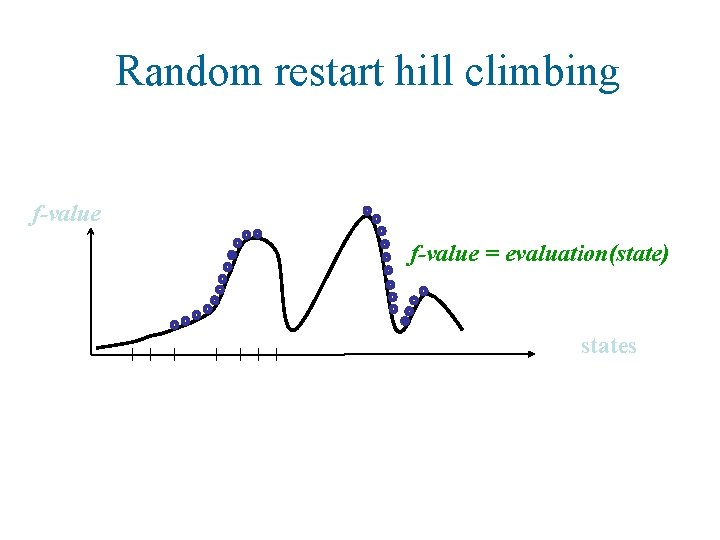
Random restart hill climbing f-value = evaluation(state) states

Randomized Iterative Improvement: • initialize search at some point of search space search steps: • with probability p, move from current search position to a randomly selected neighboring position • otherwise, move from current search position to neighboring position with better evaluation function value. • Has many variations of how to choose the randomly neighbor, and how many of them • Example: Take 100 steps in one direction (Army mistake correction) – to escape from local optima.

Simulated annealing Combinatorial search technique inspired by the physical process of annealing [Kirkpatrick et al. 1983, Cerny 1985] Outline · Select a neighbor at random. · If better than current state go there. · Otherwise, go there with some probability. · Probability goes down with time (similar to temperature cooling)

Simulated annealing e E/T

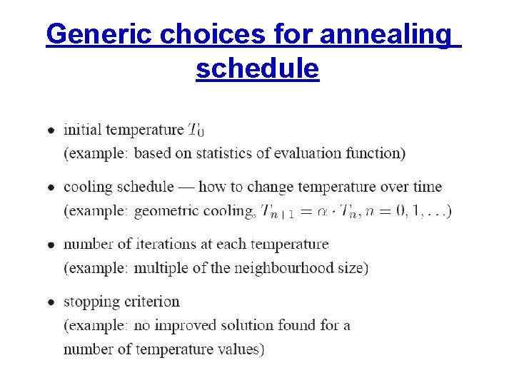
Generic choices for annealing schedule

Pseudo code function Simulated-Annealing(problem, schedule) returns solution state current Make-Node(Initial-State[problem]) for t 1 to infinity T schedule[t] // T goes downwards. if T = 0 then return current next Random-Successor(current) E f-Value[next] - f-Value[current] if E > 0 then current next else current next with probability e E/T end

Example application to the TSP [Johnson & Mc. Geoch 1997] baseline implementation: • start with random initial solution • use 2 -exchange neighborhood • simple annealing schedule; relatively poor performance improvements: • look-up table for acceptance probabilities • neighborhood pruning • low-temperature starts

Summary-Simulated Annealing. . . • is historically important • is easy to implement • has interesting theoretical properties (convergence), but these are of very limited practical relevance • achieves good performance often at the cost of substantial run-times

Tabu Search • Combinatorial search technique which heavily relies on the use of an explicit memory of the search process [Glover 1989, 1990] to guide search process • memory typically contains only specific attributes of previously seen solutions • simple tabu search strategies exploit only short term memory • more complex tabu search strategies exploit long term memory

Tabu search – exploiting short term memory • in each step, move to best neighboring solution although it may be worse than current one • to avoid cycles, tabu search tries to avoid revisiting previously seen solutions by basing the memory on attributes of recently seen solutions • tabu list stores attributes of the tl most recently visited • solutions; parameter tl is called tabu list length or tabu tenure • solutions which contain tabu attributes are forbidden

Tabu Search Problem: previously unseen solutions may be tabu use of aspiration criteria to override tabu status Stopping criteria: • all neighboring solutions are tabu • maximum number of iterations exceeded • number of iterations without improvement Robust Tabu Search [Taillard 1991], Reactive Tabu Search[Battiti & Tecchiolli 1994– 1997]

Example: Tabu Search for SAT / MAX-SAT • Neighborhood: assignments which differ in exactly one variable instantiation • Tabu attributes: variables • Tabu criterion: flipping a variable is forbidden for a given number of iterations • Aspiration criterion: if flipping a tabu variable leads to a better solution, the variable’s tabu status is overridden [Hansen & Jaumard 1990; Selman & Kautz 1994]

Genetic algorithms • Combinatorial search technique inspired by the evolution of biological species. • population of individual solutions represented as strings • individuals within population are evaluated based on their “fitness” (evaluation function value) • population is manipulated via evolutionary operators – mutation – crossover – selection

Genetic algorithms • How to generate the next generation. • 1) Selection: we select a number of states from the current generation. (we can use the fitness function in any reasonable way) • 2) crossover : select 2 states and reproduce a child. • 3) mutation: change some of the genues.

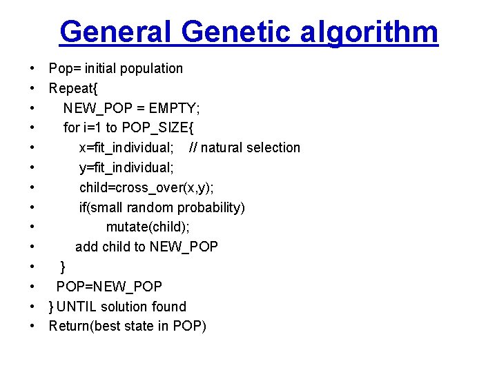
General Genetic algorithm • • • • Pop= initial population Repeat{ NEW_POP = EMPTY; for i=1 to POP_SIZE{ x=fit_individual; // natural selection y=fit_individual; child=cross_over(x, y); if(small random probability) mutate(child); add child to NEW_POP } POP=NEW_POP } UNTIL solution found Return(best state in POP)

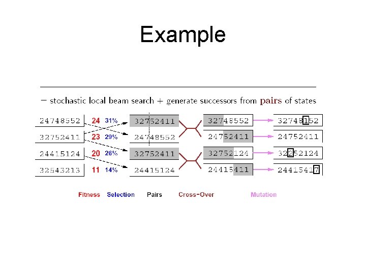
Example

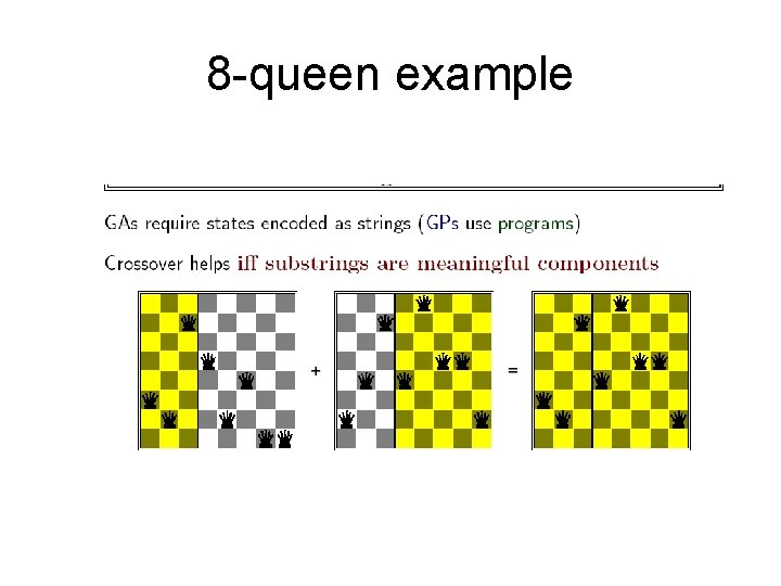
8 -queen example

Summary: Genetic Algorithms • use populations, which leads to increased search space exploration • allow for a large number of different implementation choices • typically reach best performance when using operators that are based on problem characteristics • achieve good performance on a wide range of problems