Data Stream Processing Part IV Cormode Muthukrishnan An

Data Stream Processing (Part IV) • Cormode, Muthukrishnan. “An improved data stream summary: The Count. Min sketch and its applications”, Jrnl. of Algorithms, 2005. • Datar, Gionis, Indyk, Motwani. “Maintaining Stream Statistics over Sliding Windows”, SODA’ 2002. • SURVEY-1: S. Muthukrishnan. “Data Streams: Algorithms and Applications” • SURVEY-2: Babcock et al. “Models and Issues in Data Stream Systems”, ACM PODS’ 2002.

The Streaming Model · Underlying signal: One-dimensional array A[1…N] with values A[i] all initially zero – Multi-dimensional arrays as well (e. g. , row-major) · Signal is implicitly represented via a stream of updates – j-th update is <k, c[j]> implying • A[k] : = A[k] + c[j] (c[j] can be >0, <0) · Goal: Compute functions on A[] subject to – Small space – Fast processing of updates – Fast function computation –… 2

Streaming Model: Special Cases · Time-Series Model – Only j-th updates A[j] (i. e. , A[j] : = c[j]) · Cash-Register Model – c[j] is always >= 0 (i. e. , increment-only) – Typically, c[j]=1, so we see a multi-set of items in one pass · Turnstile Model – Most general streaming model – c[j] can be >0 or <0 (i. e. , increment or decrement) · Problem difficulty varies depending on the model – E. g. , MIN/MAX in Time-Series vs. Turnstile! 3

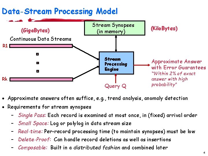
Data-Stream Processing Model (Giga. Bytes) Stream Synopses (in memory) (Kilo. Bytes) Continuous Data Streams R 1 Stream Processing Engine Rk Query Q Approximate Answer with Error Guarantees “Within 2% of exact answer with high probability” · Approximate answers often suffice, e. g. , trend analysis, anomaly detection · Requirements for stream synopses – Single Pass: Each record is examined at most once, in (fixed) arrival order – Small Space: Log or polylog in data stream size – Real-time: Per-record processing time (to maintain synopses) must be low – Delete-Proof: Can handle record deletions as well as insertions – Composable: Built in a distributed fashion and combined later 4

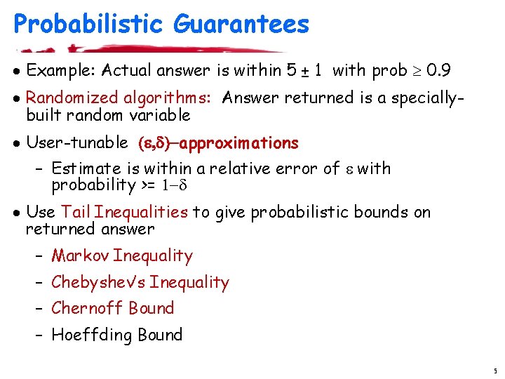
Probabilistic Guarantees · Example: Actual answer is within 5 ± 1 with prob 0. 9 · Randomized algorithms: Answer returned is a speciallybuilt random variable · User-tunable (e, d)-approximations – Estimate is within a relative error of e with probability >= 1 -d · Use Tail Inequalities to give probabilistic bounds on returned answer – Markov Inequality – Chebyshev’s Inequality – Chernoff Bound – Hoeffding Bound 5

Overview · Introduction & Motivation · Data Streaming Models & Basic Mathematical Tools · Summarization/Sketching Tools for Streams – Sampling – Linear-Projection (aka AMS) Sketches • Applications: Join/Multi-Join Queries, Wavelets – Hash (aka FM) Sketches • Applications: Distinct Values, Distinct sampling, Set Expressions 6

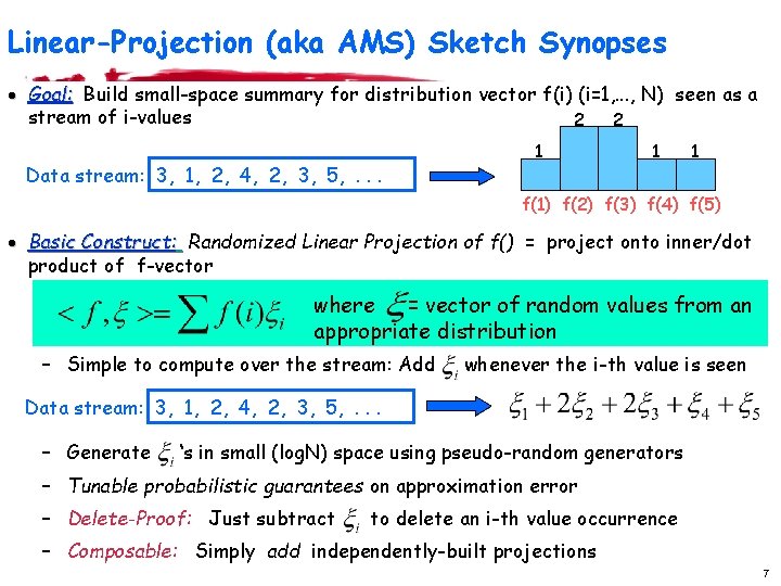
Linear-Projection (aka AMS) Sketch Synopses · Goal: Build small-space summary for distribution vector f(i) (i=1, . . . , N) seen as a stream of i-values 2 2 Data stream: 3, 1, 2, 4, 2, 3, 5, . . . 1 1 1 f(1) f(2) f(3) f(4) f(5) · Basic Construct: Randomized Linear Projection of f() = project onto inner/dot product of f-vector where = vector of random values from an appropriate distribution – Simple to compute over the stream: Add whenever the i-th value is seen Data stream: 3, 1, 2, 4, 2, 3, 5, . . . – Generate ‘s in small (log. N) space using pseudo-random generators – Tunable probabilistic guarantees on approximation error – Delete-Proof: Just subtract to delete an i-th value occurrence – Composable: Simply add independently-built projections 7

Hash (aka FM) Sketches for Distinct Value Estimation [FM 85] · Assume a hash function h(x) that maps incoming values x in [0, …, N-1] uniformly across [0, …, 2^L-1], where L = O(log. N) · Let lsb(y) denote the position of the least-significant 1 bit in the binary representation of y – A value x is mapped to lsb(h(x)) · Maintain Hash Sketch = BITMAP array of L bits, initialized to 0 – For each incoming value x, set BITMAP[ lsb(h(x)) ] = 1 x=5 h(x) = 101100 lsb(h(x)) = 2 5 4 0 0 3 0 BITMAP 2 1 0 0 8

Hash (aka FM) Sketches for Distinct Value Estimation [FM 85] · By uniformity through h(x): Prob[ BITMAP[k]=1 ] = Prob[ ]= – Assuming d distinct values: expect d/2 to map to BITMAP[0] , d/4 to map to BITMAP[1], . . . BITMAP L-1 0 0 0 position >> log(d) 0 1 0 1 1 fringe of 0/1 s around log(d) 1 1 1 position << log(d) · Let R = position of rightmost zero in BITMAP – Use as indicator of log(d) · Average several iid instances (different hash functions) to reduce estimator variance 9

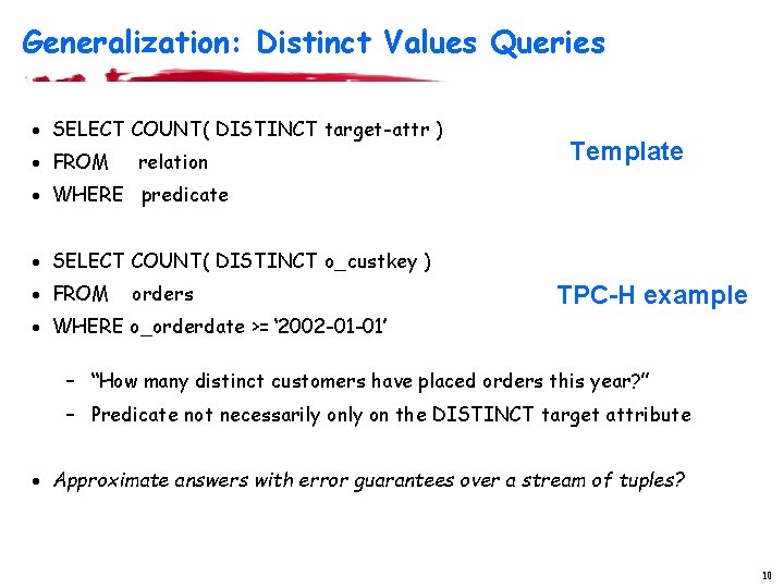
Generalization: Distinct Values Queries · SELECT COUNT( DISTINCT target-attr ) · FROM relation Template · WHERE predicate · SELECT COUNT( DISTINCT o_custkey ) · FROM orders TPC-H example · WHERE o_orderdate >= ‘ 2002 -01 -01’ – “How many distinct customers have placed orders this year? ” – Predicate not necessarily on the DISTINCT target attribute · Approximate answers with error guarantees over a stream of tuples? 10

Distinct Sampling [Gib 01] Key Ideas · Use FM-like technique to collect a specially-tailored sample over the distinct values in the stream – Use hash function mapping to sample values from the data domain!! – Uniform random sample of the distinct values – Very different from traditional random sample: each distinct value is chosen uniformly regardless of its frequency – DISTINCT query answers: simply scale up sample answer by sampling rate · To handle additional predicates – Reservoir sampling of tuples for each distinct value in the sample – Use reservoir sample to evaluate predicates 11

Processing Set Expressions over Update Streams [GGR 03] · Estimate cardinality of general set expressions over streams of updates – E. g. , number of distinct (source, dest) pairs seen at both R 1 and R 2 but not R 3? | (R 1 R 2) – R 3 | · 2 -Level Hash-Sketch (2 LHS) stream synopsis: Generalizes FM sketch – First level: buckets with exponentially-decreasing probabilities (using lsb(h(x)), as in FM) – Second level: Count-signature array (log. N+1 counters) • One “total count” for elements in first-level bucket • log. N “bit-location counts” for 1 -bits of incoming elements insert(17) lsb(h(17)) -1 for deletes!! 17 = Tot. Count +1 +1 +1 count 7 0 count 6 0 count 5 0 count 4 1 count 3 0 count 2 0 count 1 0 count 0 1 12

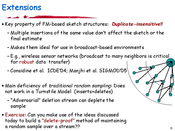
Extensions · Key property of FM-based sketch structures: Duplicate-insensitive!! – Multiple insertions of the same value don’t affect the sketch or the final estimate – Makes them ideal for use in broadcast-based environments – E. g. , wireless sensor networks (broadcast to many neighbors is critical for robust data transfer) – Considine et al. ICDE’ 04; Manjhi et al. SIGMOD’ 05 · Main deficiency of traditional random sampling: Does not work in a Turnstile Model (inserts+deletes) – “Adversarial” deletion stream can deplete the sample · Exercise: Can you make use of the ideas discussed today to build a “delete-proof” method of maintaining a random sample over a stream? ? 13

New stuff for today… · A different sketch structure for multi-sets: The Count. Min (CM) sketch · The Sliding Window model and Exponential Histograms (EHs) · Peek into distributed streaming 14

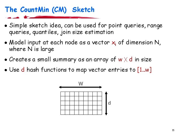
The Count. Min (CM) Sketch · Simple sketch idea, can be used for point queries, range queries, quantiles, join size estimation · Model input at each node as a vector xi of dimension N, where N is large · Creates a small summary as an array of w ╳ d in size · Use d hash functions to map vector entries to [1. . w] W d 15

CM Sketch Structure h 1(j) +xi[j] j, xi[j] hd(j) d +xi[j] w · Each entry in vector A is mapped to one bucket per row · Merge two sketches by entry-wise summation · Estimate A[j] by taking mink sketch[k, hk(j)] [Cormode, Muthukrishnan 16

CM Sketch Summary · CM sketch guarantees approximation error on point queries less than e||A||1 in size O(1/e log 1/d) – Probability of more error is less than 1 -d – Similar guarantees for range queries, quantiles, join size · Hints – Counts are biased! Can you limit the expected amount of extra “mass” at each bucket? (Use Markov) – Use Chernoff to boost the confidence for the min{} estimate · Food for thought: How do the CM sketch guarantees compare to AMS? ? 17

Sliding Window Streaming Model · Model – At every time t, a data record arrives – The record “expires” at time t+N (N is the window length) · When is it useful? – Make decisions based on “recently observed” data – Stock data – Sensor networks 18

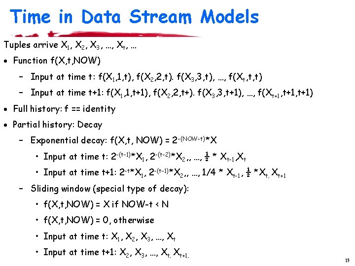
Time in Data Stream Models Tuples arrive X 1, X 2, X 3, …, Xt, … · Function f(X, t, NOW) – Input at time t: f(X 1, 1, t), f(X 2, 2, t). f(X 3, 3, t), …, f(Xt, t, t) – Input at time t+1: f(X 1, 1, t+1), f(X 2, 2, t+). f(X 3, 3, t+1), …, f(Xt+1, t+1) · Full history: f == identity · Partial history: Decay – Exponential decay: f(X, t, NOW) = 2 -(NOW-t)*X • Input at time t: 2 -(t-1)*X 1, 2 -(t-2)*X 2, , …, ½ * Xt-1, Xt • Input at time t+1: 2 -t*X 1, 2 -(t-1)*X 2, , …, 1/4 * Xt-1, ½ *Xt, Xt+1 – Sliding window (special type of decay): • f(X, t, NOW) = X if NOW-t < N • f(X, t, NOW) = 0, otherwise • Input at time t: X 1, X 2, X 3, …, Xt • Input at time t+1: X 2, X 3, …, Xt+1, 19

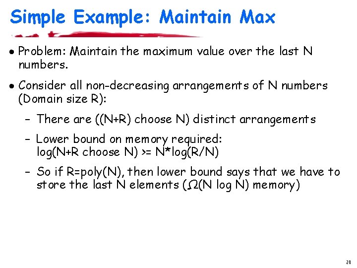
Simple Example: Maintain Max · Problem: Maintain the maximum value over the last N numbers. · Consider all non-decreasing arrangements of N numbers (Domain size R): – There are ((N+R) choose N) distinct arrangements – Lower bound on memory required: log(N+R choose N) >= N*log(R/N) – So if R=poly(N), then lower bound says that we have to store the last N elements (Ω(N log N) memory) 20

Statistics Over Sliding Windows · Bitstream: Count the number of ones [DGIM 02] – Exact solution: Θ(N) bits – Algorithm Basic. Counting: • 1 + ε approximation (relative error!) • Space: O(1/ε (log 2 N)) bits • Time: O(log N) worst case, O(1) amortized per record – Lower Bound: • Space: Ω(1/ε (log 2 N)) bits 21

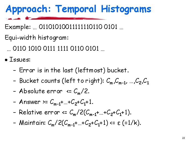
Approach: Temporal Histograms Example: … 01101010011111110110 0101 … Equi-width histogram: … 0110 1010 0111 1111 0110 0101 … · Issues: – Error is in the last (leftmost) bucket. – Bucket counts (left to right): Cm, Cm-1, …, C 2, C 1 – Absolute error <= Cm/2. – Answer >= Cm-1+…+C 2+C 1+1. – Relative error <= Cm/2(Cm-1+…+C 2+C 1+1). – Maintain: Cm/2(Cm-1+…+C 2+C 1+1) <= ε (=1/k). 22

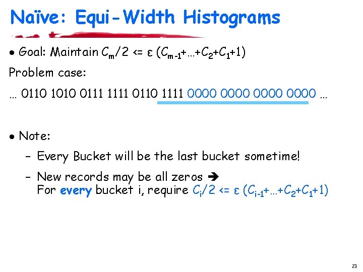
Naïve: Equi-Width Histograms · Goal: Maintain Cm/2 <= ε (Cm-1+…+C 2+C 1+1) Problem case: … 0110 1010 0111 1111 0110 1111 0000 … · Note: – Every Bucket will be the last bucket sometime! – New records may be all zeros For every bucket i, require Ci/2 <= ε (Ci-1+…+C 2+C 1+1) 23

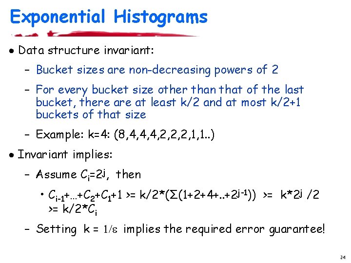
Exponential Histograms · Data structure invariant: – Bucket sizes are non-decreasing powers of 2 – For every bucket size other than that of the last bucket, there at least k/2 and at most k/2+1 buckets of that size – Example: k=4: (8, 4, 4, 4, 2, 2, 2, 1, 1. . ) · Invariant implies: – Assume Ci=2 j, then • Ci-1+…+C 2+C 1+1 >= k/2*(Σ(1+2+4+. . +2 j-1)) >= k*2 j /2 >= k/2*Ci – Setting k = 1/e implies the required error guarantee! 24

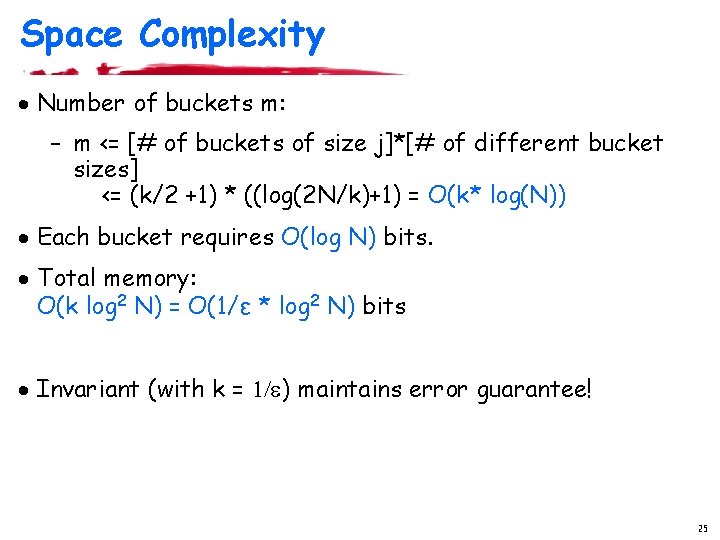
Space Complexity · Number of buckets m: – m <= [# of buckets of size j]*[# of different bucket sizes] <= (k/2 +1) * ((log(2 N/k)+1) = O(k* log(N)) · Each bucket requires O(log N) bits. · Total memory: O(k log 2 N) = O(1/ε * log 2 N) bits · Invariant (with k = 1/e) maintains error guarantee! 25

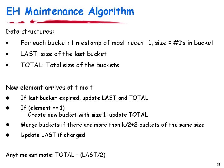
EH Maintenance Algorithm Data structures: · For each bucket: timestamp of most recent 1, size = #1’s in bucket · LAST: size of the last bucket · TOTAL: Total size of the buckets New element arrives at time t l If last bucket expired, update LAST and TOTAL l If (element == 1) Create new bucket with size 1; update TOTAL l Merge buckets if there are more than k/2+2 buckets of the same size l Update LAST if changed Anytime estimate: TOTAL – (LAST/2) 26

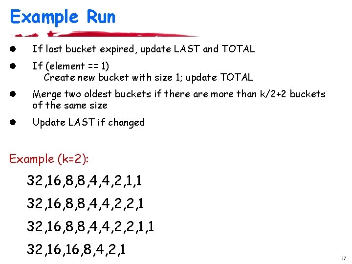
Example Run l If last bucket expired, update LAST and TOTAL l If (element == 1) Create new bucket with size 1; update TOTAL l Merge two oldest buckets if there are more than k/2+2 buckets of the same size l Update LAST if changed Example (k=2): 32, 16, 8, 8, 4, 4, 2, 1, 1 32, 16, 8, 8, 4, 4, 2, 2, 1, 1 32, 16, 8, 4, 2, 1 27

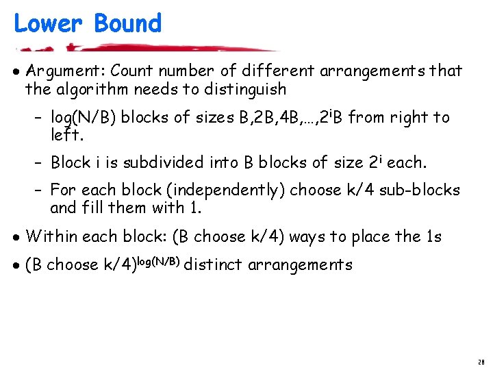
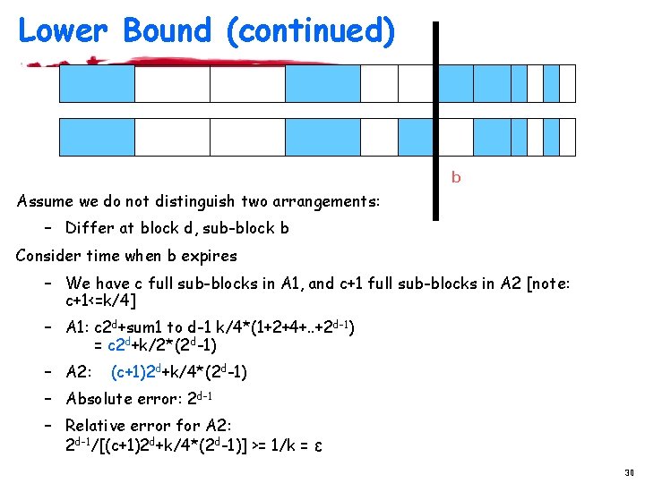
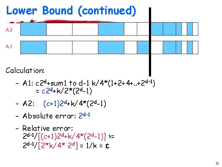
Lower Bound · Argument: Count number of different arrangements that the algorithm needs to distinguish – log(N/B) blocks of sizes B, 2 B, 4 B, …, 2 i. B from right to left. – Block i is subdivided into B blocks of size 2 i each. – For each block (independently) choose k/4 sub-blocks and fill them with 1. · Within each block: (B choose k/4) ways to place the 1 s · (B choose k/4)log(N/B) distinct arrangements 28

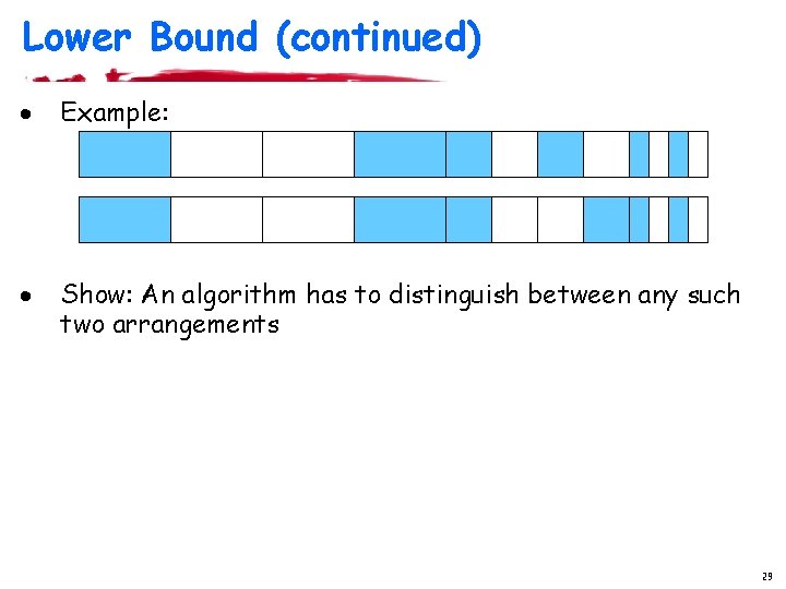
Lower Bound (continued) · Example: · Show: An algorithm has to distinguish between any such two arrangements 29

Lower Bound (continued) b Assume we do not distinguish two arrangements: – Differ at block d, sub-block b Consider time when b expires – We have c full sub-blocks in A 1, and c+1 full sub-blocks in A 2 [note: c+1<=k/4] – A 1: c 2 d+sum 1 to d-1 k/4*(1+2+4+. . +2 d-1) = c 2 d+k/2*(2 d-1) – A 2: (c+1)2 d+k/4*(2 d-1) – Absolute error: 2 d-1 – Relative error for A 2: 2 d-1/[(c+1)2 d+k/4*(2 d-1)] >= 1/k = ε 30

Lower Bound (continued) A 2 A 1 Calculation: – A 1: c 2 d+sum 1 to d-1 k/4*(1+2+4+. . +2 d-1) = c 2 d+k/2*(2 d-1) – A 2: (c+1)2 d+k/4*(2 d-1) – Absolute error: 2 d-1 – Relative error: 2 d-1/[(c+1)2 d+k/4*(2 d-1)] >= 2 d-1/[2*k/4* 2 d] = 1/k = ε 31

The Power of EHs · Counter for N items = O(log. N) space · EH = e-approximate counter over sliding window of N items that requires O(1/ε * log 2 N) space – O(1/e log. N) penalty for (approx) sliding-window counting · Can plugin EH-counters to counter-based streaming methods work in sliding-window model!! – Examples: histograms, CM-sketches, … · Complication: counting is now e-approximate – Account for that in analysis 32

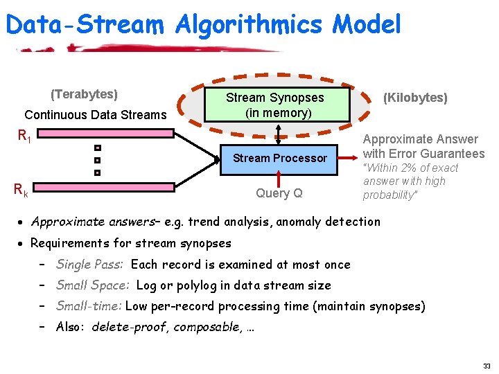
Data-Stream Algorithmics Model (Terabytes) Continuous Data Streams Stream Synopses (in memory) R 1 Stream Processor Rk Query Q (Kilobytes) Approximate Answer with Error Guarantees “Within 2% of exact answer with high probability” · Approximate answers– e. g. trend analysis, anomaly detection · Requirements for stream synopses – Single Pass: Each record is examined at most once – Small Space: Log or polylog in data stream size – Small-time: Low per-record processing time (maintain synopses) – Also: delete-proof, composable, … 33

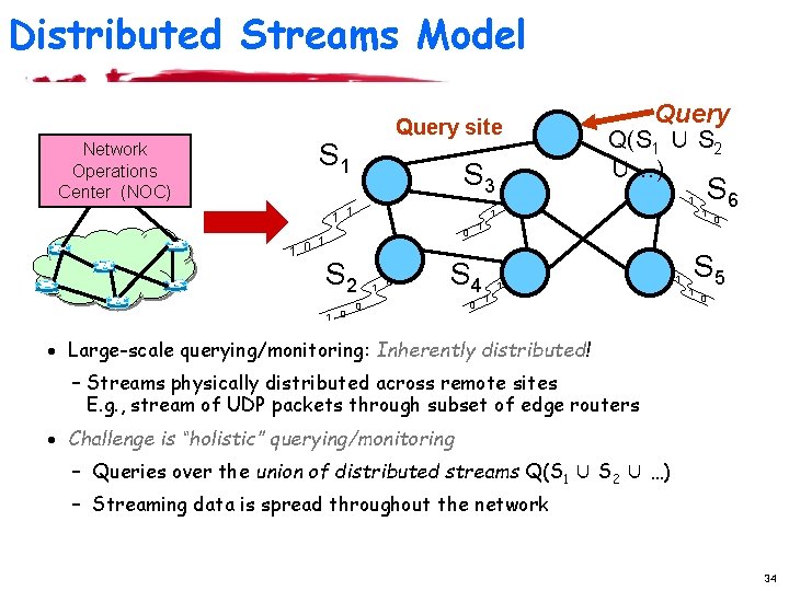
Distributed Streams Model Network Operations Center (NOC) Query site S 1 S 3 1 1 0 Q(S 1 ∪ S 2 ∪…) 1 1 S 2 1 0 S 4 0 S 6 1 1 0 Query 0 1 1 1 0 S 5 1 0 · Large-scale querying/monitoring: Inherently distributed! – Streams physically distributed across remote sites E. g. , stream of UDP packets through subset of edge routers · Challenge is “holistic” querying/monitoring – Queries over the union of distributed streams Q(S 1 ∪ S 2 ∪ …) – Streaming data is spread throughout the network 34

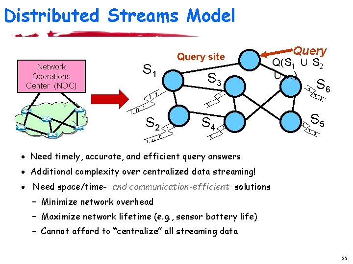
Distributed Streams Model Network Operations Center (NOC) Query site S 1 S 3 1 1 0 Q(S 1 ∪ S 2 ∪…) 1 1 S 2 0 1 0 S 6 1 1 0 Query S 4 0 1 1 1 0 S 5 1 0 · Need timely, accurate, and efficient query answers · Additional complexity over centralized data streaming! · Need space/time- and communication-efficient solutions – Minimize network overhead – Maximize network lifetime (e. g. , sensor battery life) – Cannot afford to “centralize” all streaming data 35

Conclusions · Querying and finding patterns in massive streams is a real problem with many real-world applications · Fundamentally rethink data-management issues under stringent constraints – Single-pass algorithms with limited memory resources · A lot of progress in the last few years – Algorithms, system models & architectures • Giga. Scope (AT&T), Aurora (Brandeis/Brown/MIT), Niagara (Wisconsin), STREAM (Stanford), Telegraph (Berkeley) · Commercial acceptance still lagging, but will most probably grow in coming years – Specialized systems (e. g. , fraud detection, network monitoring), but still far from “DSMSs” 36