Data Stream Processing Part I Alon Matias Szegedy

Data Stream Processing (Part I) • Alon, , Matias, Szegedy. “The space complexity of approximating the frequency moments”, ACM STOC’ 1996. • Alon, Gibbons, Matias, Szegedy. “Tracking Join and Self-join Sizes in Limited Storage”, ACM PODS’ 1999. • SURVEY-1: S. Muthukrishnan. “Data Streams: Algorithms and Applications” • SURVEY-2: Babcock et al. “Models and Issues in Data Stream Systems”, ACM PODS’ 2002.

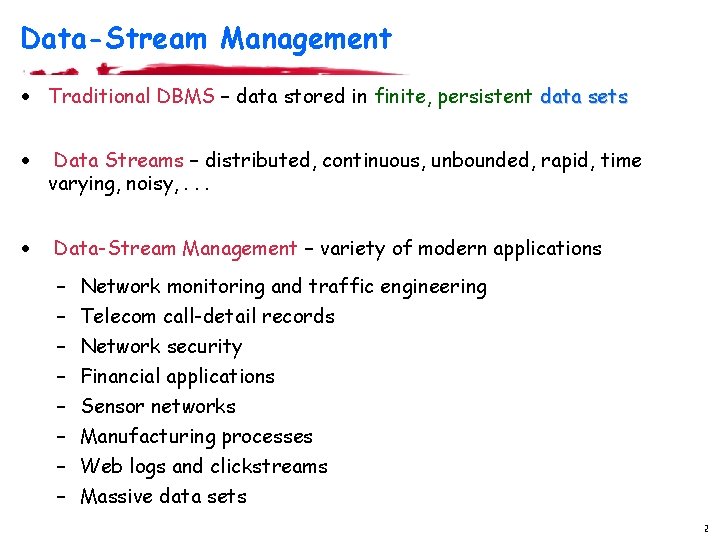
Data-Stream Management · Traditional DBMS – data stored in finite, persistent data sets · Data Streams – distributed, continuous, unbounded, rapid, time varying, noisy, . . . · Data-Stream Management – variety of modern applications – – – – Network monitoring and traffic engineering Telecom call-detail records Network security Financial applications Sensor networks Manufacturing processes Web logs and clickstreams Massive data sets 2

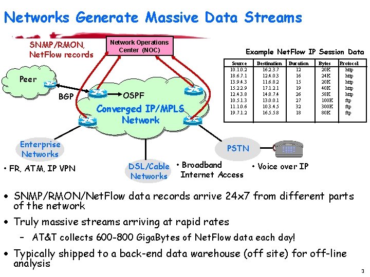
Networks Generate Massive Data Streams SNMP/RMON, Net. Flow records Network Operations Center (NOC) Example Net. Flow IP Session Data Source 10. 1. 0. 2 18. 6. 7. 1 13. 9. 4. 3 15. 2. 2. 9 12. 4. 3. 8 10. 5. 1. 3 11. 1. 0. 6 19. 7. 1. 2 Peer BGP Enterprise Networks • FR, ATM, IP VPN OSPF Converged IP/MPLS Network Destination 16. 2. 3. 7 12. 4. 0. 3 11. 6. 8. 2 17. 1. 2. 1 14. 8. 7. 4 13. 0. 0. 1 10. 3. 4. 5 16. 5. 5. 8 Duration 12 16 15 19 26 27 32 18 Bytes 20 K 24 K 20 K 40 K 58 K 100 K 300 K 80 K Protocol http http ftp ftp PSTN DSL/Cable • Broadband • Voice over IP Internet Access Networks · SNMP/RMON/Net. Flow data records arrive 24 x 7 from different parts of the network · Truly massive streams arriving at rapid rates – AT&T collects 600 -800 Giga. Bytes of Net. Flow data each day! · Typically shipped to a back-end data warehouse (off site) for off-line analysis 3

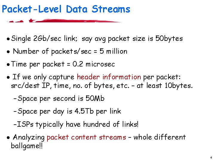
Packet-Level Data Streams · Single 2 Gb/sec link; say avg packet size is 50 bytes · Number of packets/sec = 5 million · Time per packet = 0. 2 microsec · If we only capture header information per packet: src/dest IP, time, no. of bytes, etc. – at least 10 bytes. – Space per second is 50 Mb – Space per day is 4. 5 Tb per link – ISPs typically have hundred of links! · Analyzing packet content streams – whole different ballgame!! 4

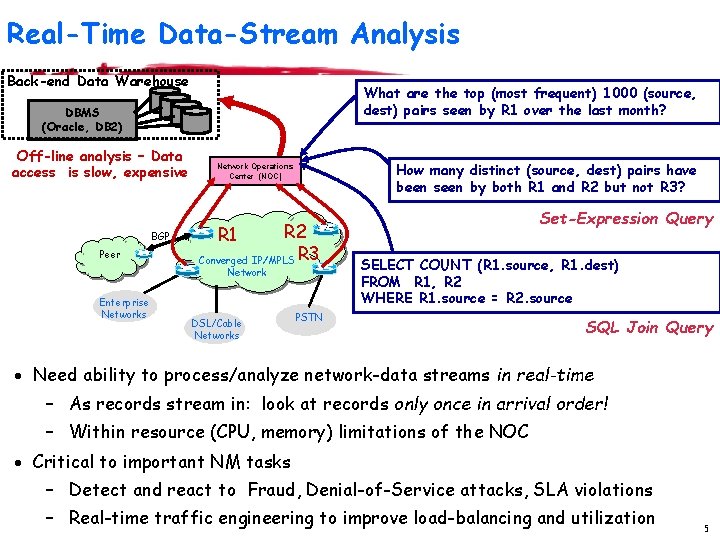
Real-Time Data-Stream Analysis Back-end Data Warehouse What are the top (most frequent) 1000 (source, dest) pairs seen by R 1 over the last month? DBMS (Oracle, DB 2) Off-line analysis – Data access is slow, expensive BGP Peer How many distinct (source, dest) pairs have been seen by both R 1 and R 2 but not R 3? Network Operations Center (NOC) R 2 Converged IP/MPLS R 3 R 1 Network Enterprise Networks Set-Expression Query DSL/Cable Networks SELECT COUNT (R 1. source, R 1. dest) FROM R 1, R 2 WHERE R 1. source = R 2. source PSTN SQL Join Query · Need ability to process/analyze network-data streams in real-time – As records stream in: look at records only once in arrival order! – Within resource (CPU, memory) limitations of the NOC · Critical to important NM tasks – Detect and react to Fraud, Denial-of-Service attacks, SLA violations – Real-time traffic engineering to improve load-balancing and utilization 5

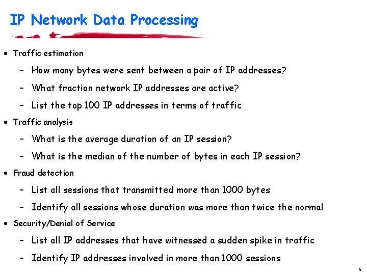
IP Network Data Processing · Traffic estimation – How many bytes were sent between a pair of IP addresses? – What fraction network IP addresses are active? – List the top 100 IP addresses in terms of traffic · Traffic analysis – What is the average duration of an IP session? – What is the median of the number of bytes in each IP session? · Fraud detection – List all sessions that transmitted more than 1000 bytes – Identify all sessions whose duration was more than twice the normal · Security/Denial of Service – List all IP addresses that have witnessed a sudden spike in traffic – Identify IP addresses involved in more than 1000 sessions 6

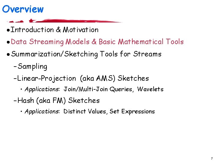
Overview · Introduction & Motivation · Data Streaming Models & Basic Mathematical Tools · Summarization/Sketching Tools for Streams – Sampling – Linear-Projection (aka AMS) Sketches • Applications: Join/Multi-Join Queries, Wavelets – Hash (aka FM) Sketches • Applications: Distinct Values, Set Expressions 7

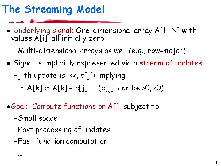
The Streaming Model · Underlying signal: One-dimensional array A[1…N] with values A[i] all initially zero – Multi-dimensional arrays as well (e. g. , row-major) · Signal is implicitly represented via a stream of updates – j-th update is <k, c[j]> implying • A[k] : = A[k] + c[j] (c[j] can be >0, <0) · Goal: Compute functions on A[] subject to – Small space – Fast processing of updates – Fast function computation –… 8

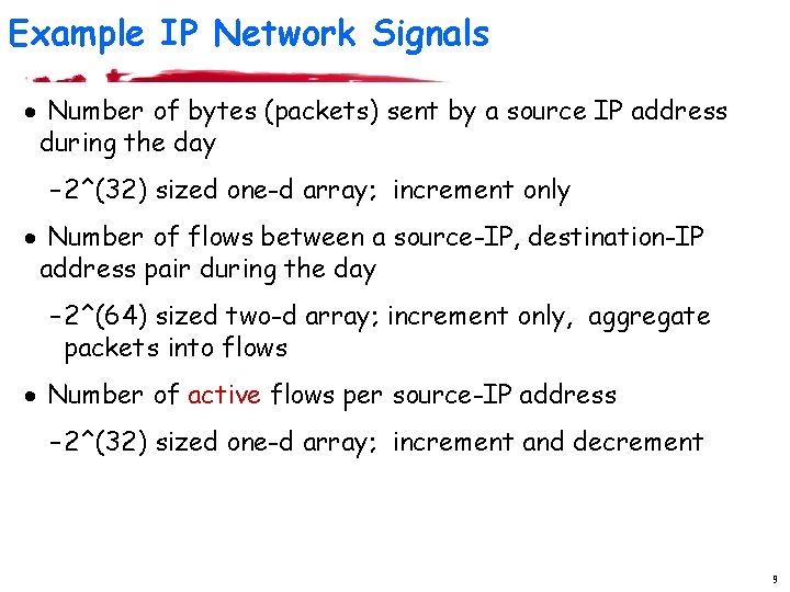
Example IP Network Signals · Number of bytes (packets) sent by a source IP address during the day – 2^(32) sized one-d array; increment only · Number of flows between a source-IP, destination-IP address pair during the day – 2^(64) sized two-d array; increment only, aggregate packets into flows · Number of active flows per source-IP address – 2^(32) sized one-d array; increment and decrement 9

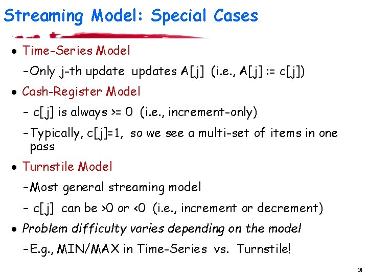
Streaming Model: Special Cases · Time-Series Model – Only j-th updates A[j] (i. e. , A[j] : = c[j]) · Cash-Register Model – c[j] is always >= 0 (i. e. , increment-only) – Typically, c[j]=1, so we see a multi-set of items in one pass · Turnstile Model – Most general streaming model – c[j] can be >0 or <0 (i. e. , increment or decrement) · Problem difficulty varies depending on the model – E. g. , MIN/MAX in Time-Series vs. Turnstile! 10

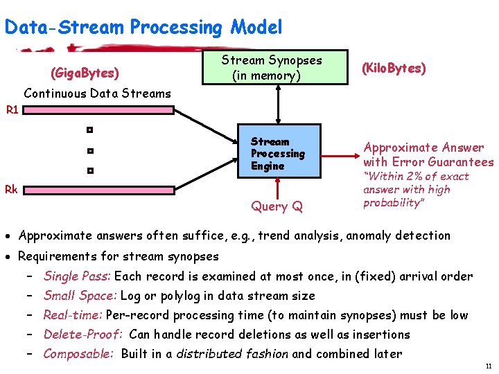
Data-Stream Processing Model (Giga. Bytes) Stream Synopses (in memory) (Kilo. Bytes) Continuous Data Streams R 1 Stream Processing Engine Rk Query Q Approximate Answer with Error Guarantees “Within 2% of exact answer with high probability” · Approximate answers often suffice, e. g. , trend analysis, anomaly detection · Requirements for stream synopses – Single Pass: Each record is examined at most once, in (fixed) arrival order – Small Space: Log or polylog in data stream size – Real-time: Per-record processing time (to maintain synopses) must be low – Delete-Proof: Can handle record deletions as well as insertions – Composable: Built in a distributed fashion and combined later 11

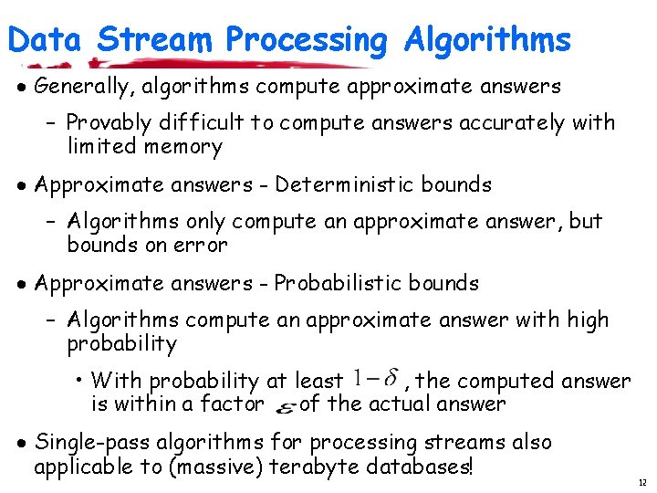
Data Stream Processing Algorithms · Generally, algorithms compute approximate answers – Provably difficult to compute answers accurately with limited memory · Approximate answers - Deterministic bounds – Algorithms only compute an approximate answer, but bounds on error · Approximate answers - Probabilistic bounds – Algorithms compute an approximate answer with high probability • With probability at least , the computed answer is within a factor of the actual answer · Single-pass algorithms for processing streams also applicable to (massive) terabyte databases! 12

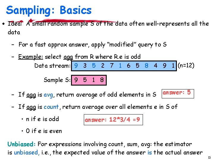
Sampling: Basics · Idea: A small random sample S of the data often well-represents all the data – For a fast approx answer, apply “modified” query to S – Example: select agg from R where R. e is odd Data stream: 9 3 5 2 7 1 6 5 8 4 9 1 (n=12) Sample S: 9 5 1 8 – If agg is avg, return average of odd elements in S answer: 5 – If agg is count, return average over all elements e in S of • n if e is odd answer: 12*3/4 =9 • 0 if e is even Unbiased: For expressions involving count, sum, avg: the estimator is unbiased, i. e. , the expected value of the answer is the actual answer 13

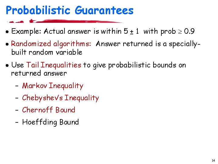
Probabilistic Guarantees · Example: Actual answer is within 5 ± 1 with prob 0. 9 · Randomized algorithms: Answer returned is a speciallybuilt random variable · Use Tail Inequalities to give probabilistic bounds on returned answer – Markov Inequality – Chebyshev’s Inequality – Chernoff Bound – Hoeffding Bound 14

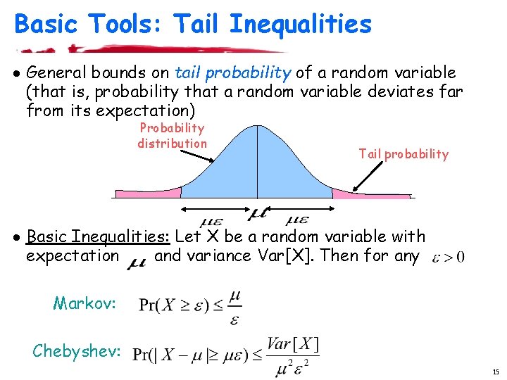
Basic Tools: Tail Inequalities · General bounds on tail probability of a random variable (that is, probability that a random variable deviates far from its expectation) Probability distribution Tail probability · Basic Inequalities: Let X be a random variable with expectation and variance Var[X]. Then for any Markov: Chebyshev: 15

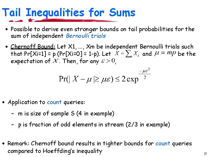
Tail Inequalities for Sums · Possible to derive even stronger bounds on tail probabilities for the sum of independent Bernoulli trials · Chernoff Bound: Let X 1, . . . , Xm be independent Bernoulli trials such that Pr[Xi=1] = p (Pr[Xi=0] = 1 -p). Let and be the expectation of. Then, for any , · Application to count queries: – m is size of sample S (4 in example) – p is fraction of odd elements in stream (2/3 in example) · Remark: Chernoff bound results in tighter bounds for count queries compared to Hoeffding’s inequality 17

Overview · Introduction & Motivation · Data Streaming Models & Basic Mathematical Tools · Summarization/Sketching Tools for Streams – Sampling – Linear-Projection (aka AMS) Sketches • Applications: Join/Multi-Join Queries, Wavelets – Hash (aka FM) Sketches • Applications: Distinct Values, Set Expressions 18

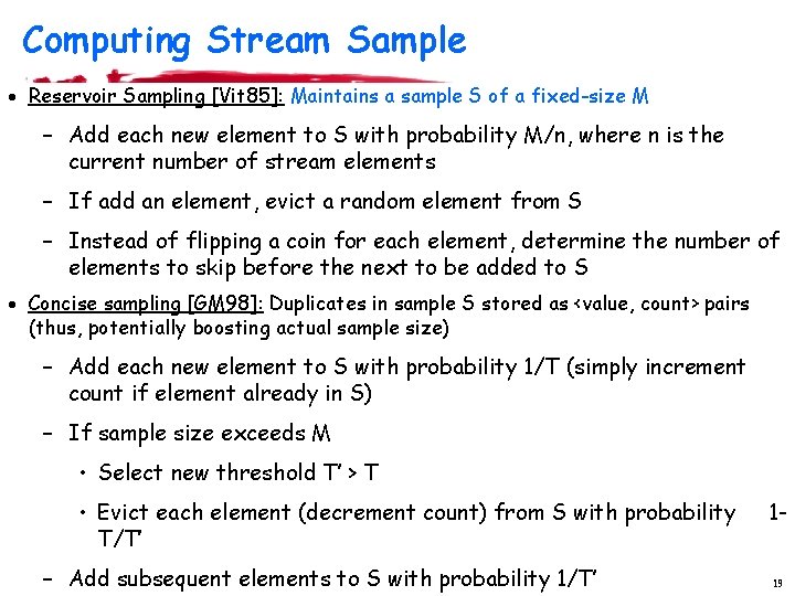
Computing Stream Sample · Reservoir Sampling [Vit 85]: Maintains a sample S of a fixed-size M – Add each new element to S with probability M/n, where n is the current number of stream elements – If add an element, evict a random element from S – Instead of flipping a coin for each element, determine the number of elements to skip before the next to be added to S · Concise sampling [GM 98]: Duplicates in sample S stored as <value, count> pairs (thus, potentially boosting actual sample size) – Add each new element to S with probability 1/T (simply increment count if element already in S) – If sample size exceeds M • Select new threshold T’ > T • Evict each element (decrement count) from S with probability T/T’ – Add subsequent elements to S with probability 1/T’ 119

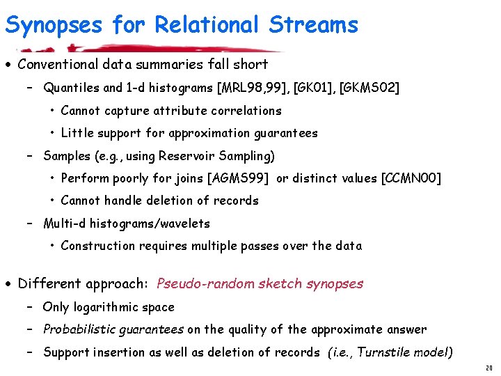
Synopses for Relational Streams · Conventional data summaries fall short – Quantiles and 1 -d histograms [MRL 98, 99], [GK 01], [GKMS 02] • Cannot capture attribute correlations • Little support for approximation guarantees – Samples (e. g. , using Reservoir Sampling) • Perform poorly for joins [AGMS 99] or distinct values [CCMN 00] • Cannot handle deletion of records – Multi-d histograms/wavelets • Construction requires multiple passes over the data · Different approach: Pseudo-random sketch synopses – Only logarithmic space – Probabilistic guarantees on the quality of the approximate answer – Support insertion as well as deletion of records (i. e. , Turnstile model) 20

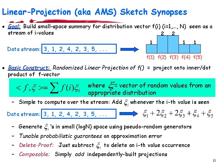
Linear-Projection (aka AMS) Sketch Synopses · Goal: Build small-space summary for distribution vector f(i) (i=1, . . . , N) seen as a stream of i-values 2 2 Data stream: 3, 1, 2, 4, 2, 3, 5, . . . 1 1 1 f(1) f(2) f(3) f(4) f(5) · Basic Construct: Randomized Linear Projection of f() = project onto inner/dot product of f-vector where = vector of random values from an appropriate distribution – Simple to compute over the stream: Add whenever the i-th value is seen Data stream: 3, 1, 2, 4, 2, 3, 5, . . . – Generate ‘s in small (log. N) space using pseudo-random generators – Tunable probabilistic guarantees on approximation error – Delete-Proof: Just subtract to delete an i-th value occurrence – Composable: Simply add independently-built projections 21

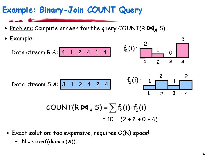
Example: Binary-Join COUNT Query · Problem: Compute answer for the query COUNT(R · Example: A 3 2 1 Data stream R. A: 4 1 2 4 1 Data stream S. A: 3 1 2 4 0 3 2 1 1 = 10 S) 2 2 4 1 3 2 4 (2 + 0 + 6) · Exact solution: too expensive, requires O(N) space! – N = sizeof(domain(A)) 22

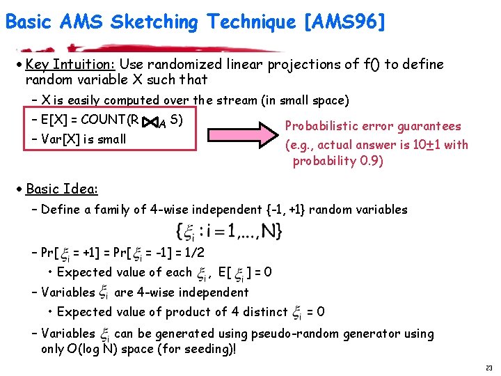
Basic AMS Sketching Technique [AMS 96] · Key Intuition: Use randomized linear projections of f() to define random variable X such that – X is easily computed over the stream (in small space) – E[X] = COUNT(R – Var[X] is small A S) Probabilistic error guarantees (e. g. , actual answer is 10± 1 with probability 0. 9) · Basic Idea: – Define a family of 4 -wise independent {-1, +1} random variables – Pr[ = +1] = Pr[ = -1] = 1/2 • Expected value of each – Variables , E[ ]=0 are 4 -wise independent • Expected value of product of 4 distinct =0 – Variables can be generated using pseudo-random generator using only O(log N) space (for seeding)! 23

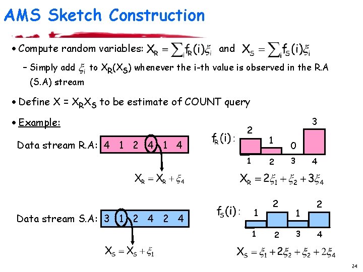
AMS Sketch Construction · Compute random variables: – Simply add (S. A) stream and to XR(XS) whenever the i-th value is observed in the R. A · Define X = XRXS to be estimate of COUNT query · Example: 3 2 1 Data stream R. A: 4 1 2 4 1 Data stream S. A: 3 1 2 4 0 3 2 1 1 2 2 4 1 3 2 4 24

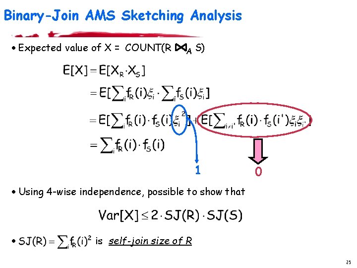
Binary-Join AMS Sketching Analysis · Expected value of X = COUNT(R A S) 1 0 · Using 4 -wise independence, possible to show that · is self-join size of R 25