More StreamMining Counting Distinct Elements Computing Moments Frequent

More Stream-Mining Counting Distinct Elements Computing “Moments” Frequent Itemsets Elephants and Troops Exponentially Decaying Windows 1

Counting Distinct Elements u. Problem: a data stream consists of elements chosen from a set of size n. Maintain a count of the number of distinct elements seen so far. u. Obvious approach: maintain the set of elements seen. 2

Applications u. How many different words are found among the Web pages being crawled at a site? w Unusually low or high numbers could indicate artificial pages (spam? ). u. How many different Web pages does each customer request in a week? 3

Using Small Storage u. Real Problem: what if we do not have space to store the complete set? u. Estimate the count in an unbiased way. u. Accept that the count may be in error, but limit the probability that the error is large. 4

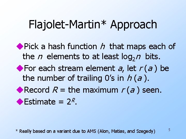
Flajolet-Martin* Approach u. Pick a hash function h that maps each of the n elements to at least log 2 n bits. u. For each stream element a, let r (a ) be the number of trailing 0’s in h (a ). u. Record R = the maximum r (a ) seen. u. Estimate = 2 R. * Really based on a variant due to AMS (Alon, Matias, and Szegedy) 5

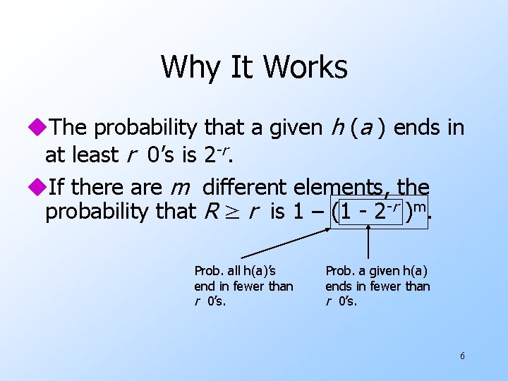
Why It Works u. The probability that a given h (a ) ends in at least r 0’s is 2 -r. u. If there are m different elements, the probability that R ≥ r is 1 – (1 - 2 -r )m. Prob. all h(a)’s end in fewer than r 0’s. Prob. a given h(a) ends in fewer than r 0’s. 6

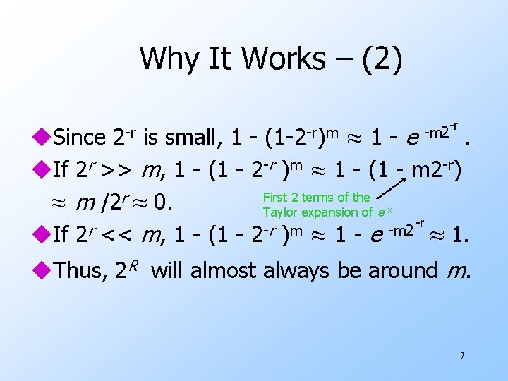
Why It Works – (2) -r u. Since is small, 1 ≈1 -e. u. If 2 r >> m, 1 - (1 - 2 -r )m ≈ 1 - (1 - m 2 -r) First 2 terms of the ≈ m /2 r ≈ 0. Taylor expansion of e -r r r m -m 2 u. If 2 << m, 1 - (1 - 2 ) ≈ 1 - e ≈ 1. 2 -r (1 -2 -r)m -m 2 x u. Thus, 2 R will almost always be around m. 7

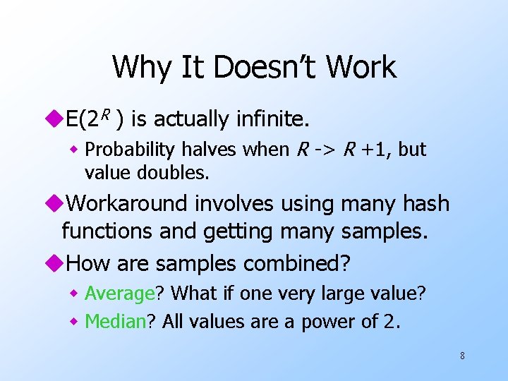
Why It Doesn’t Work u. E(2 R ) is actually infinite. w Probability halves when R -> R +1, but value doubles. u. Workaround involves using many hash functions and getting many samples. u. How are samples combined? w Average? What if one very large value? w Median? All values are a power of 2. 8

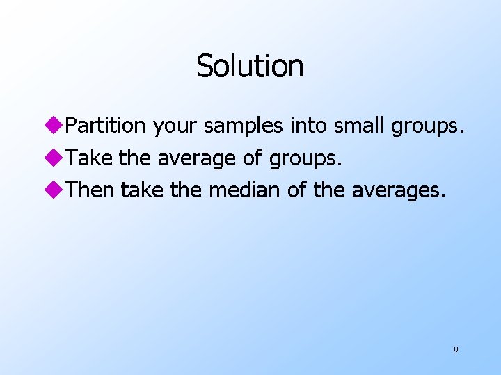
Solution u. Partition your samples into small groups. u. Take the average of groups. u. Then take the median of the averages. 9

Generalization: Moments u. Suppose a stream has elements chosen from a set of n values. u. Let mi be the number of times value i occurs. u. The k th moment is the sum of (mi )k over all i. 10

Special Cases u 0 th moment = number of different elements in the stream. w The problem just considered. u 1 st moment = count of the numbers of elements = length of the stream. w Easy to compute. u 2 nd moment = surprise number = a measure of how uneven the distribution is. 11

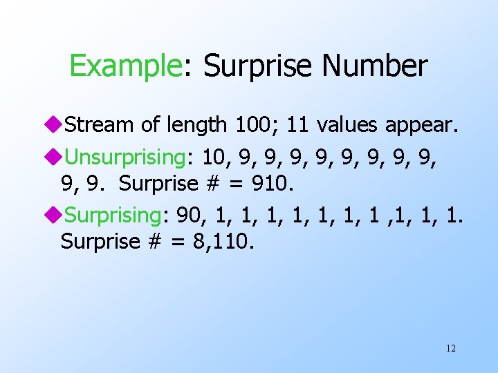
Example: Surprise Number u. Stream of length 100; 11 values appear. u. Unsurprising: 10, 9, 9, 9. Surprise # = 910. u. Surprising: 90, 1, 1, 1, 1. Surprise # = 8, 110. 12

AMS Method u. Works for all moments; gives an unbiased estimate. u. We’ll just concentrate on 2 nd moment. u. Based on calculation of many random variables X. w Each requires a count in main memory, so number is limited. 13

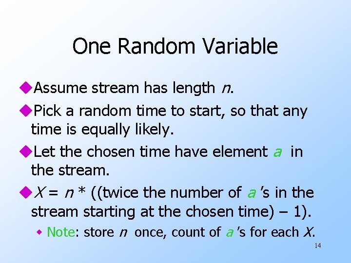
One Random Variable u. Assume stream has length n. u. Pick a random time to start, so that any time is equally likely. u. Let the chosen time have element a in the stream. u. X = n * ((twice the number of a ’s in the stream starting at the chosen time) – 1). w Note: store n once, count of a ’s for each X. 14

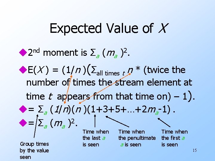
Expected Value of X u 2 nd moment is Σa (ma )2. u. E(X ) = (1/n )(Σall times t n * (twice the number of times the stream element at time t appears from that time on) – 1). u= Σa (1/n)(n )(1+3+5+…+2 ma-1). u= Σa ( m a ) 2. Group times by the value seen Time when the last a is seen Time when the penultimate a is seen Time when the first a is seen 15

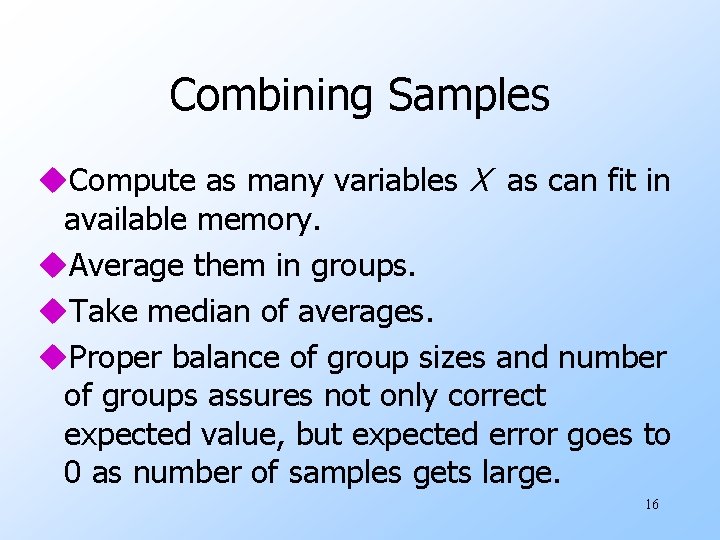
Combining Samples u. Compute as many variables X as can fit in available memory. u. Average them in groups. u. Take median of averages. u. Proper balance of group sizes and number of groups assures not only correct expected value, but expected error goes to 0 as number of samples gets large. 16

Problem: Streams Never End u. We assumed there was a number n, the number of positions in the stream. u. But real streams go on forever, so n is a variable – the number of inputs seen so far. 17

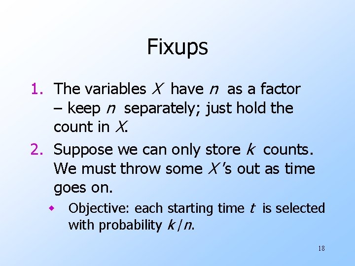
Fixups 1. The variables X have n as a factor – keep n separately; just hold the count in X. 2. Suppose we can only store k counts. We must throw some X ’s out as time goes on. w Objective: each starting time t is selected with probability k /n. 18

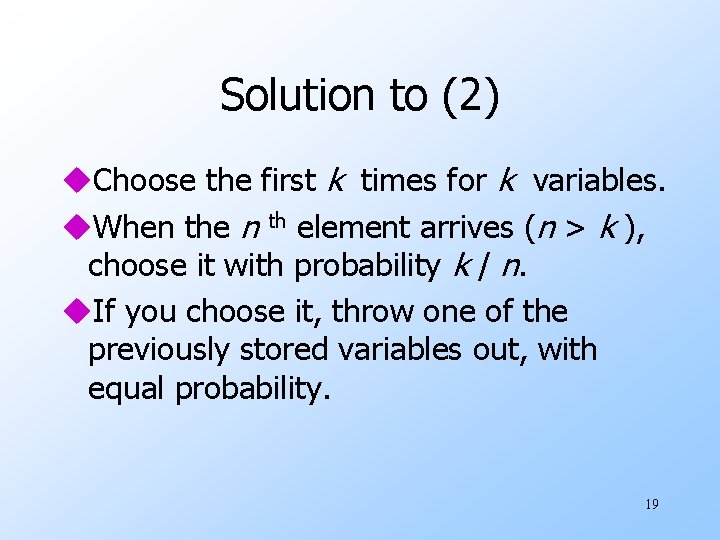
Solution to (2) u. Choose the first k times for k variables. u. When the n th element arrives (n > k ), choose it with probability k / n. u. If you choose it, throw one of the previously stored variables out, with equal probability. 19

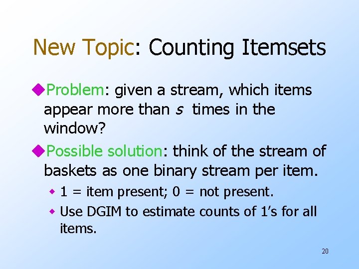
New Topic: Counting Itemsets u. Problem: given a stream, which items appear more than s times in the window? u. Possible solution: think of the stream of baskets as one binary stream per item. w 1 = item present; 0 = not present. w Use DGIM to estimate counts of 1’s for all items. 20

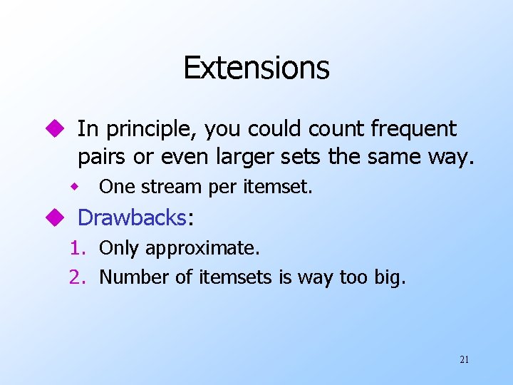
Extensions u In principle, you could count frequent pairs or even larger sets the same way. w One stream per itemset. u Drawbacks: 1. Only approximate. 2. Number of itemsets is way too big. 21

Approaches 1. “Elephants and troops”: a heuristic way to converge on unusually strongly connected itemsets. 2. Exponentially decaying windows: a heuristic for selecting likely frequent itemsets. 22

Elephants and Troops u. When Sergey Brin wasn’t worrying about Google, he tried the following experiment. u. Goal: find unusually correlated sets of words. w “High Correlation ” = frequency of occurrence of set >> product of frequencies of members. 23

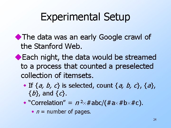
Experimental Setup u. The data was an early Google crawl of the Stanford Web. u. Each night, the data would be streamed to a process that counted a preselected collection of itemsets. w If {a, b, c} is selected, count {a, b, c}, {a}, {b}, and {c}. w “Correlation” = n 2 #abc/(#a #b #c). • n = number of pages. 24

After Each Night’s Processing. . . 1. Find the most correlated sets counted. 2. Construct a new collection of itemsets to count the next night. w All the most correlated sets (“winners ”). w Pairs of a word in some winner and a random word. w Winners combined in various ways. 25 w Some random pairs.

After a Week. . . u. The pair {“elephants”, “troops”} came up as the big winner. u. Why? It turns out that Stanford students were playing a Punic-War simulation game internationally, where moves were sent by Web pages. 26

New Topic: Mining Streams Versus Mining DB’s u. Unlike mining databases, mining streams doesn’t have a fixed answer. u. We’re really mining in the “Stat” point of view, e. g. , “Which itemsets are frequent in the underlying model that generates the stream? ” 27

Stationarity Our assumptions make a big difference: 1. Is the model stationary ? u I. e. , are the same statistics used throughout all time to generate the stream? 2. Or does the frequency of generating given items or itemsets change over time? 28

Some Options for Frequent Itemsets 1. Run periodic experiments, like E&T. u Like SON – itemset is a candidate if it is found frequent on any “day. ” u Good for stationary statistics. 2. Frame the problem as finding all frequent itemsets in an “exponentially decaying window. ” u Good for nonstationary statistics. 29

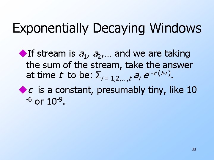
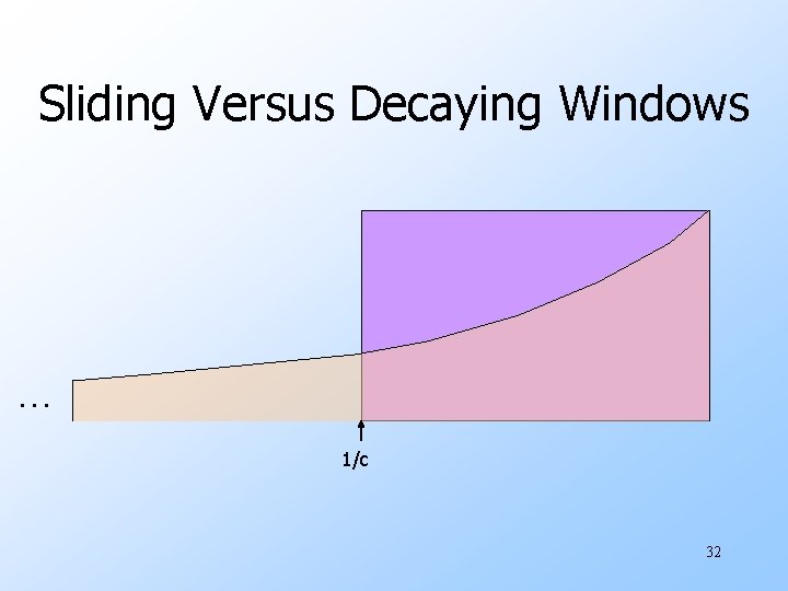
Exponentially Decaying Windows u. If stream is a 1, a 2, … and we are taking the sum of the stream, take the answer at time t to be: Σi = 1, 2, …, t ai e -c (t-i ). uc is a constant, presumably tiny, like 10 -6 or 10 -9. 30

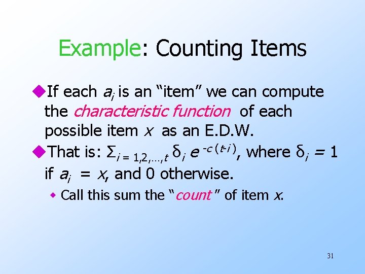
Example: Counting Items u. If each ai is an “item” we can compute the characteristic function of each possible item x as an E. D. W. u. That is: Σi = 1, 2, …, t δi e -c (t-i ), where δi = 1 if ai = x, and 0 otherwise. w Call this sum the “count ” of item x. 31

Sliding Versus Decaying Windows . . . 1/c 32

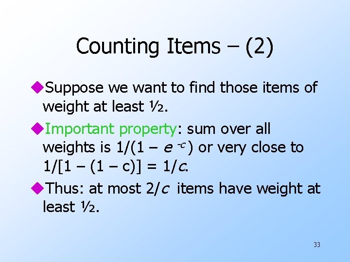
Counting Items – (2) u. Suppose we want to find those items of weight at least ½. u. Important property: sum over all weights is 1/(1 – e -c ) or very close to 1/[1 – (1 – c)] = 1/c. u. Thus: at most 2/c items have weight at least ½. 33

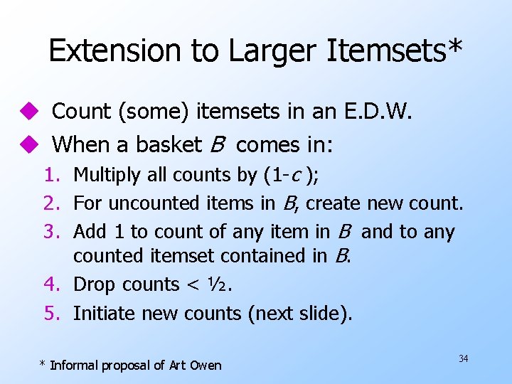
Extension to Larger Itemsets* u Count (some) itemsets in an E. D. W. u When a basket B comes in: 1. Multiply all counts by (1 -c ); 2. For uncounted items in B, create new count. 3. Add 1 to count of any item in B and to any counted itemset contained in B. 4. Drop counts < ½. 5. Initiate new counts (next slide). * Informal proposal of Art Owen 34

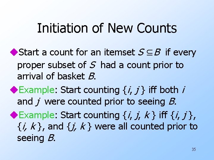
Initiation of New Counts u. Start a count for an itemset S ⊆B if every proper subset of S had a count prior to arrival of basket B. u. Example: Start counting {i, j } iff both i and j were counted prior to seeing B. u. Example: Start counting {i, j, k } iff {i, j }, {i, k }, and {j, k } were all counted prior to seeing B. 35

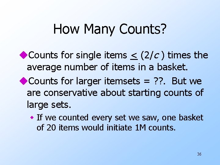
How Many Counts? u. Counts for single items < (2/c ) times the average number of items in a basket. u. Counts for larger itemsets = ? ? . But we are conservative about starting counts of large sets. w If we counted every set we saw, one basket of 20 items would initiate 1 M counts. 36