Finding Frequent Items in Data Streams Moses Charikar


- Slides: 37

Finding Frequent Items in Data Streams Moses Charikar Princeton Un. , Google Inc. Kevin Chen UC Berkeley, Google Inc. Martin Franch-Colton Rutgers Un. , Google Inc. Presented by Amir Rothschild

Presenting: ¡ ¡ ¡ 1 -pass algorithm for estimating the most frequent items in a data stream using very limited storage space. The algorithm achieves especially good space bounds for Zipfian distribution 2 -pass algorithm for estimating the items with the largest change in frequency between two data streams.

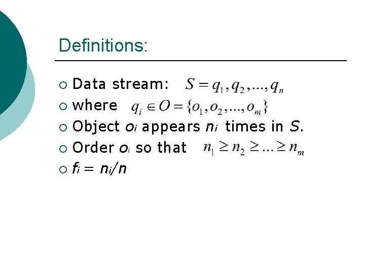
Definitions: Data stream: ¡ where ¡ Object oi appears ni times in S. ¡ Order oi so that ¡ fi = ni/n ¡

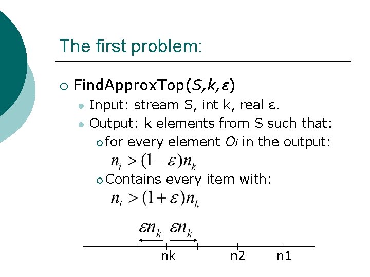
The first problem: ¡ Find. Approx. Top(S, k, ε) l l Input: stream S, int k, real ε. Output: k elements from S such that: ¡ for every element Oi in the output: ¡ Contains every item with: nk n 2 n 1

Clarifications: This is not the problem discussed last week! ¡ Sampling algorithm does not give any bounds for this version of the problem. ¡

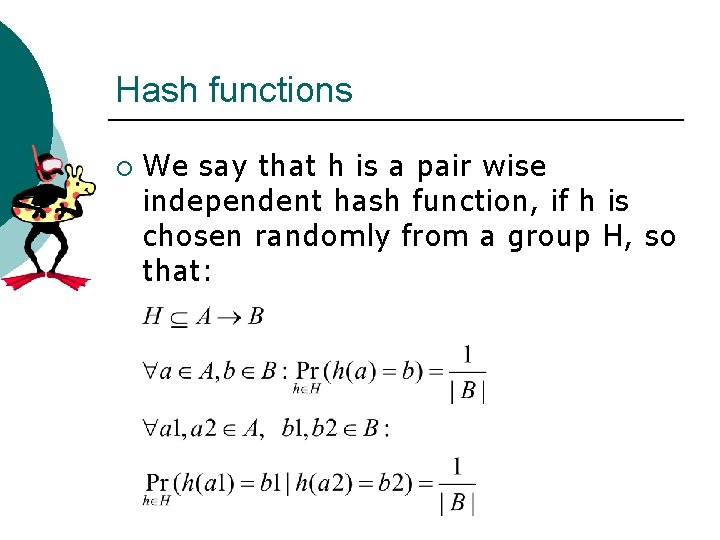
Hash functions ¡ We say that h is a pair wise independent hash function, if h is chosen randomly from a group H, so that:

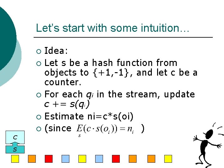
Let’s start with some intuition… Idea: ¡ Let s be a hash function from objects to {+1, -1}, and let c be a counter. ¡ For each qi in the stream, update c += s(qi) ¡ Estimate ni=c*s(oi) ¡ (since ) ¡ C S

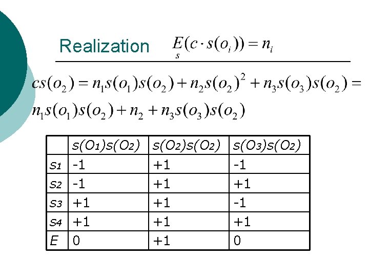
Realization s 1 s 2 s 3 s 4 E s(O 1)s(O 2) -1 -1 +1 +1 0 s(O 2) +1 +1 +1 s(O 3)s(O 2) -1 +1 0

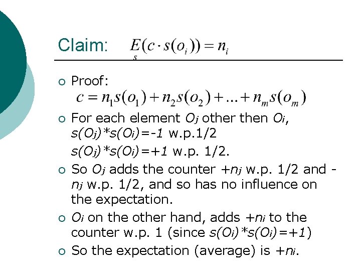
Claim: ¡ Proof: ¡ For each element Oj other then Oi, s(Oj)*s(Oi)=-1 w. p. 1/2 s(Oj)*s(Oi)=+1 w. p. 1/2. So Oj adds the counter +nj w. p. 1/2 and nj w. p. 1/2, and so has no influence on the expectation. Oi on the other hand, adds +ni to the counter w. p. 1 (since s(Oi)*s(Oi)=+1) So the expectation (average) is +ni. ¡ ¡ ¡

That’s not enough: The variance is very high. ¡ O(m) objects have estimates that are wrong by more then the variance. ¡

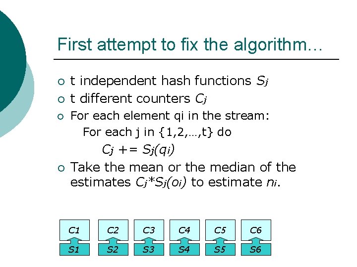
First attempt to fix the algorithm… ¡ ¡ t independent hash functions Sj t different counters Cj For each element qi in the stream: For each j in {1, 2, …, t} do Cj += Sj(qi) Take the mean or the median of the estimates Cj*Sj(oi) to estimate ni. C 1 C 2 C 3 C 4 C 5 C 6 S 1 S 2 S 3 S 4 S 5 S 6

Still not enough ¡ Collisions with high frequency elements like O 1 can spoil most estimates of lower frequency elements, as Ok.

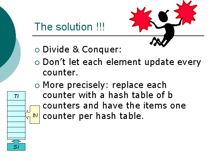
The solution !!! Divide & Conquer: ¡ Don’t let each element update every counter. ¡ More precisely: replace each counter with a hash table of b counters and have the items one hi counter per hash table. ¡ Ti Ci Si

Let’s start working… Presenting the Count. Sketch algorithm…

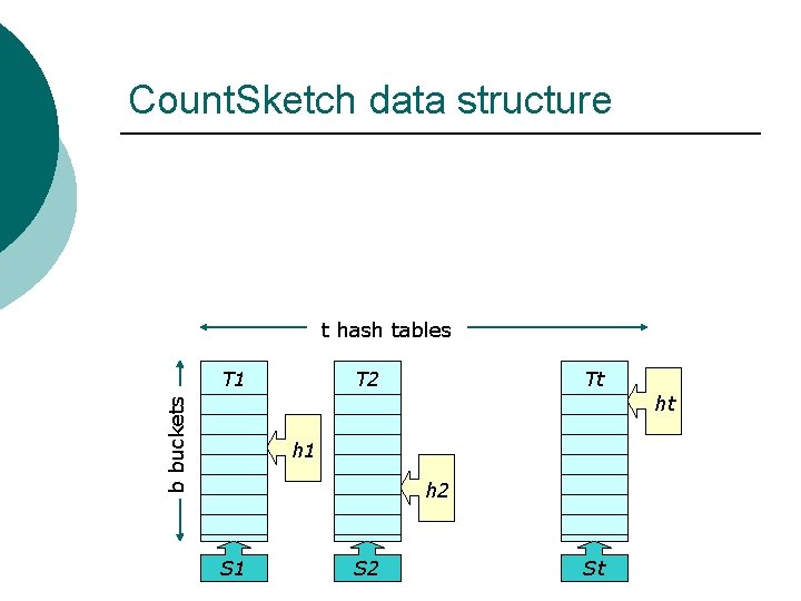
Count. Sketch data structure t hash tables h 1 T 1 h 2 T 2 ht Tt b buckets ht h 1 h 2 S 1 S 2 St

The Count. Sketch data structure ¡ ¡ ¡ Define Count. Skatch d. s. as follows: Let t and b be parameters with values determined later. h 1, …, ht – hash functions O -> {1, 2, …, b}. T 1, …, Tt – arrays of b counters. S 1, …, St – hash functions from objects O to {+1, -1}. From now on, define : hi[oj] : = Ti[hi(oj)]

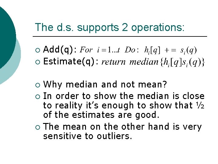
The d. s. supports 2 operations: Add(q): ¡ Estimate(q): ¡ Why median and not mean? ¡ In order to show the median is close to reality it’s enough to show that ½ of the estimates are good. ¡ The mean on the other hand is very sensitive to outliers. ¡

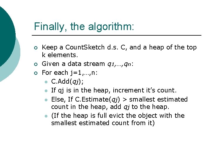
Finally, the algorithm: ¡ ¡ ¡ Keep a Count. Sketch d. s. C, and a heap of the top k elements. Given a data stream q 1, …, qn: For each j=1, …, n: l C. Add(qj); l If qj is in the heap, increment it’s count. l Else, If C. Estimate(qj) > smallest estimated count in the heap, add qj to the heap. l (If the heap is full evict the object with the smallest estimated count from it)

And now for the hard part: Algorithms analysis

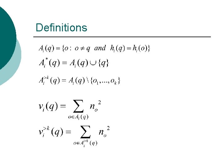
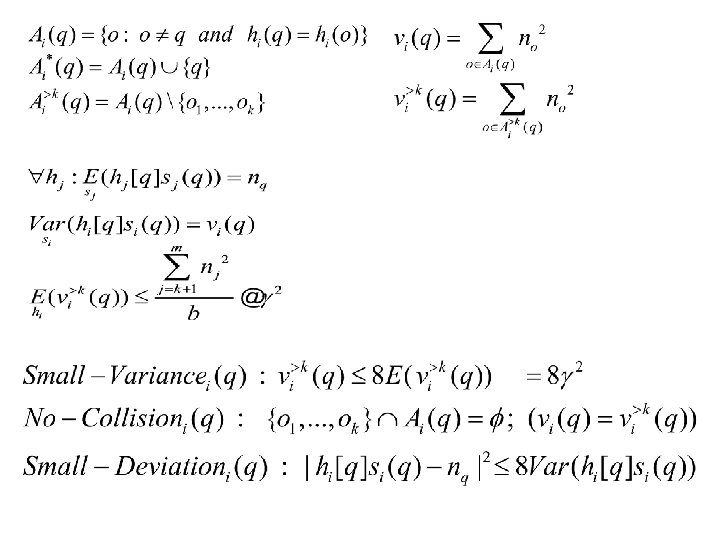
Definitions

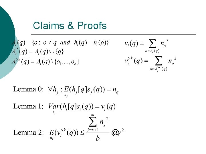
Claims & Proofs


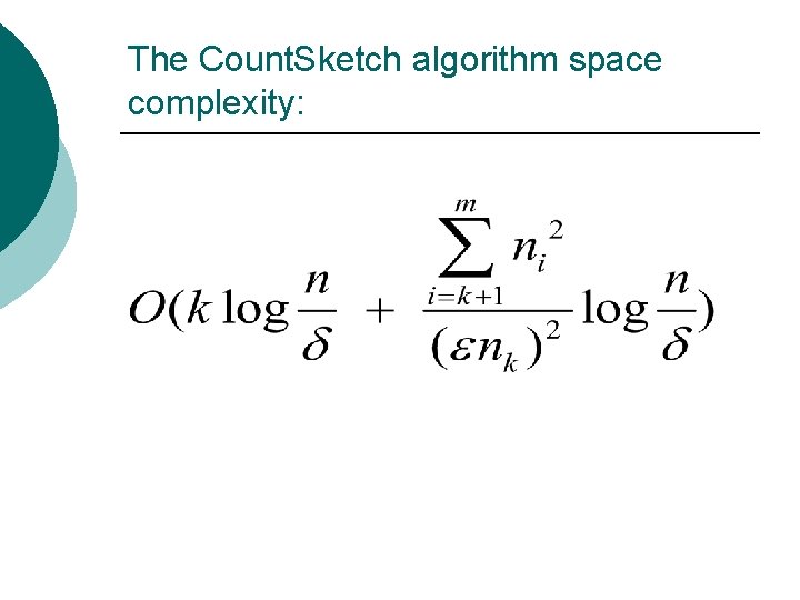
The Count. Sketch algorithm space complexity:

Zipfian distribution Analysis of the Count. Sketch algorithm for Zipfian distribution

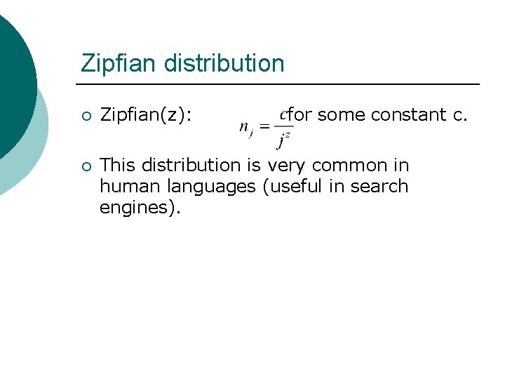
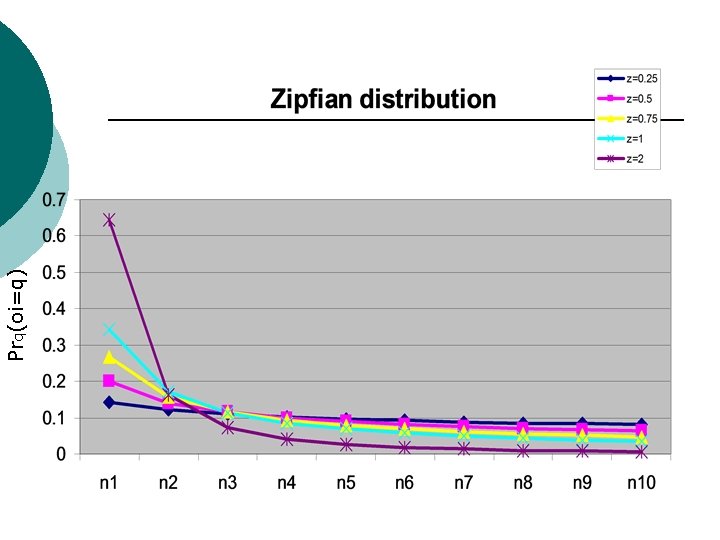
Zipfian distribution ¡ Zipfian(z): for some constant c. ¡ This distribution is very common in human languages (useful in search engines).

Prq(oi=q)

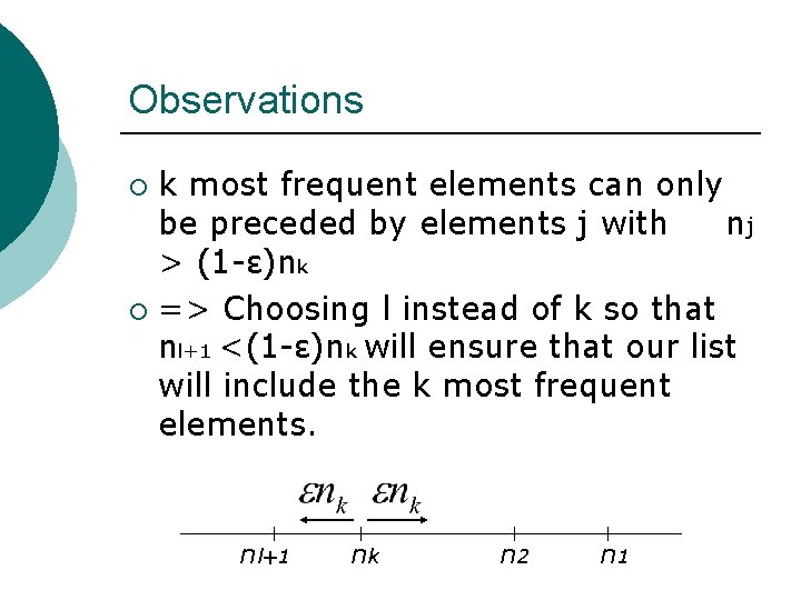
Observations k most frequent elements can only be preceded by elements j with nj > (1 -ε)nk ¡ => Choosing l instead of k so that nl+1 <(1 -ε)nk will ensure that our list will include the k most frequent elements. ¡ nl+1 nk n 2 n 1

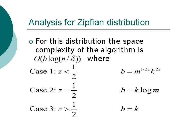
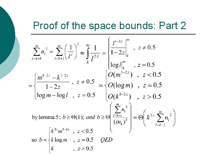
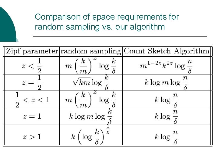
Analysis for Zipfian distribution ¡ For this distribution the space complexity of the algorithm is where:

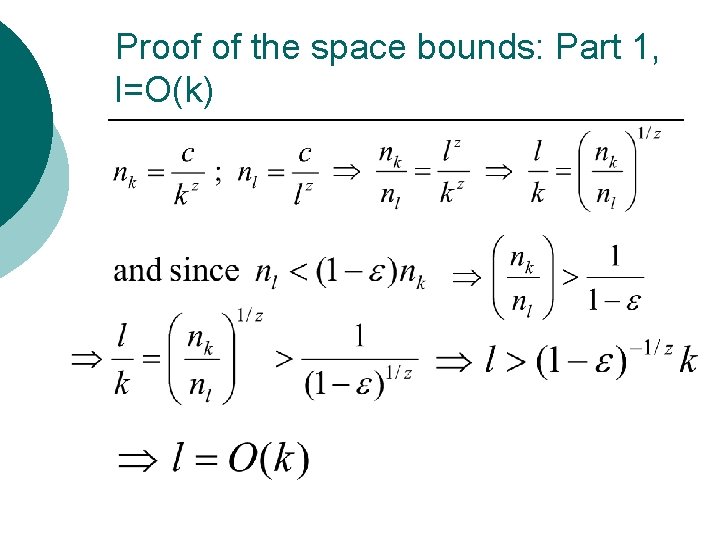
Proof of the space bounds: Part 1, l=O(k)

Proof of the space bounds: Part 2

Comparison of space requirements for random sampling vs. our algorithm

Yet another algorithm which uses Count. Sketch d. s. Finding items with largest frequency change

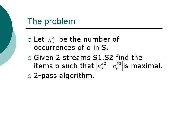
The problem Let be the number of occurrences of o in S. ¡ Given 2 streams S 1, S 2 find the items o such that is maximal. ¡ 2 -pass algorithm. ¡

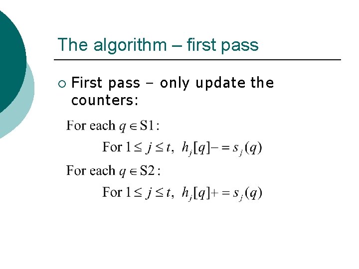
The algorithm – first pass ¡ First pass – only update the counters:

The algorithm – second pass ¡ Pass over S 1 and S 2 and:

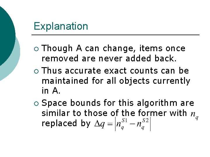
Explanation Though A can change, items once removed are never added back. ¡ Thus accurate exact counts can be maintained for all objects currently in A. ¡ Space bounds for this algorithm are similar to those of the former with replaced by ¡
