Frequent Pattern Mining Association Rules 1 Outline l

Frequent Pattern Mining - Association Rules 1

Outline l 何謂頻繁樣式的勘測 （frequent pattern mining）? l Association Rules Problem Overview Ø Large itemsets l Association Rules Algorithms (頻繁樣式的勘測方法) Ø Apriori, … Ø Sampling Ø Partitioning Ø Parallel Algorithms l Comparing Techniques l Incremental Algorithms l Advanced AR Techniques l 植基於條件式的（Constraint-based）頻繁樣式勘測 Ming-Yen Lin, IECS, FCU 2

F. P. M. 是data mining的基本功能/ 作 l 許多data mining task的基礎 Ø Association rules, correlation, causality Ø sequential patterns, temporal/cyclic association, partial periodicity Ø spatial and multimedia patterns Ø associative classification Ø cluster analysis Ø iceberg cube, … l 廣泛的應用 Ø 購物籃分析 Ø 交叉行銷 Ø 型錄設計 Ø 行銷活動分析 Ø web log (click stream)分析, DNA sequence analysis, … Ming-Yen Lin, IECS, FCU 3

基本觀念: 頻繁項目集 l 項目集 Itemset X={x 1, …, xk} Ø 例：{A, C}, {B, E, F}, {C, E} l 項目集的支持度( support） Pattern = set of items Øs(A) = 3/4 l 頻繁項目集: 符合最小支持度（ m. s. : minimum support ）的項目集 l 勘測頻繁樣式: 找出所有的頻繁樣式 Transaction-id Items bought 10 A, B, C 20 A, C 30 A, D 40 B, E, F 4 Ming-Yen Lin, IECS, FCU

Example: Market Basket Data l Items frequently purchased together: Bread Peanut. Butter l Uses: ØPlacement ØAdvertising ØSales ØCoupons l Objective: increase sales and reduce costs 5 Ming-Yen Lin, IECS, FCU

Association Rule Definitions l Set of items: I={I 1, I 2, …, Im} l Transactions: D={t 1, t 2, …, tn}, tj I l Itemset: {Ii 1, Ii 2, …, Iik} I l Support of an itemset: Percentage of transactions which contain that itemset. l Large (Frequent) itemset: Itemset whose number of occurrences is above a threshold. 6 Ming-Yen Lin, IECS, FCU

Association Rules Example I = { Beer, Bread, Jelly, Milk, Peanut. Butter} Support of {Bread, Peanut. Butter} is 60% Large (frequent) itemset: …(if ms=50%) Ming-Yen Lin, IECS, FCU 7

Association Rule Definitions l Association Rule (AR): implication X Y where X, Y I and X Y = ; l Support of AR (s) X Y: Percentage of transactions that contain X Y l Confidence of AR (a) X Y: Ratio of number of transactions that contain X Y to the number that contain X 8 Ming-Yen Lin, IECS, FCU

Association Rules Ex (cont’d) 9 Ming-Yen Lin, IECS, FCU

基本觀念: 關聯規則 Transaction-id Items bought 10 A, B, C 20 A, C 30 A, D 40 B, E, F l 關聯規則的勘測: 頻繁 項目集找出後，決定「 有興趣的」項目集之間 的關係 Ø 信賴度 confidence, c, 某交易 Customer buys both Customer buys diaper 如果包含 X ，此交易同時 會包含Y的條件機率 Ø 支持度 support, s, 某交易包 含 X Y的機率 l m. s. = 50%, m. c. = 50% Customer buys beer Ming-Yen Lin, IECS, FCU Ø A C (50%, 66. 7%) Ø C A (50%, 100%) m. s. : minimum support 最小支持度 m. c. : minimum confidence 最小信賴度 10

探勘關聯規則（例） Min. support 50% Min. confidence 50% Transaction-id Items bought 10 A, B, C 20 A, C Frequent pattern Support 30 A, D {A} 75% 40 B, E, F {B} 50% {C} 50% {A, C} 50% rule A C: support = support({A} {C}) = 50% confidence = support({A} {C})/support({A}) = 66. 6% 11 Ming-Yen Lin, IECS, FCU

Association Rule Problem l Given a set of items I={I 1, I 2, …, Im} and a database of transactions D={t 1, t 2, …, tn} where ti={Ii 1, Ii 2, …, Iik} and Iij I, the Association Rule Problem is to identify all association rules X Y with a minimum support and confidence. ØLink Analysis l NOTE: Support of X Y is same as support of X Y. 12 Ming-Yen Lin, IECS, FCU

Association Rule Techniques 1. Find Large Itemsets. n bottleneck n Apriori, … 2. Generate rules from frequent itemsets. 13 Ming-Yen Lin, IECS, FCU

Generate Rules 14 Ming-Yen Lin, IECS, FCU

頻繁樣式的勘測方法 l Well-Known Algorithm: Apriori l Apriori ØMethod overview ØProperty ØData Structure l 加速Apriori 方法 (Same framework) l 改進Apriori 方法 (Different framework) Ø不產生「候選樣式」的探勘方法 15 Ming-Yen Lin, IECS, FCU

Apriori l Large Itemset Property: (downward closure) Any subset of a large itemset is large. l Contrapositive: If an itemset is not large, none of its supersets are large. 16 Ming-Yen Lin, IECS, FCU

Large Itemset Property 17 Ming-Yen Lin, IECS, FCU

Apriori 方法實例 Database Tid 10 20 30 40 L 2 Items A, C, D B, C, E A, B, C, E B, E Itemset {A, C} {B, E} {C, E} C 3 Ming-Yen Lin, IECS, FCU m. s. = 2 C 1 1 st scan C 2 sup 2 2 3 2 Itemset {B, C, E} Itemset {A} {B} {C} {D} {E} Itemset {A, B} {A, C} {A, E} {B, C} {B, E} {C, E} 3 rd scan sup 2 3 3 1 3 sup 1 2 3 2 L 3 L 1 C 2 2 nd scan Itemset {B, C, E} sup 以count表示，未以%表示 Itemset {A} {B} {C} {E} sup 2 3 3 3 Itemset {A, B} {A, C} {A, E} {B, C} {B, E} {C, E} sup 2 19

Apriori 演算法細節 L 1 = {frequent items}; k = 1 ; if Lk = stop ; Ck+1 = 由 Lk 產生; 對資料庫 D 中每一個交易 t 執行 所有包含於 t 的、 Ck+1中的 candidate的個數 (support count) 加一 Lk+1 = Ck+1之candidate滿足最小支持者 (minimum support) k = k +1 ; 答案： Lk的聯集; l Lk : 大小為 k 的 frequent itemset l Ck: 大小為 k 的candidate itemset 20 Ming-Yen Lin, IECS, FCU

Apriori 關鍵細節 I l. Ck+1 = 由 Lk 產生; ØStep 1: self-joining Lk （ Lk 自交） ØStep 2: pruning（消去不可能者） l 例：L 3={abc, abd, ace, bcd}依序排好 ØSelf-joining: L 3*L 3 nabcd： 由 abc and abd nacde：由 acd and ace ØPruning: n消去 acde : 因 ade 不在 L 3 l C 4={abcd} 21 Ming-Yen Lin, IECS, FCU

Apriori 關鍵細節 II l 所有包含於 t 的 candidate的count加一; 難在 哪？ Ø candidate的總個數太多 Ø 各個 t中包含不止一個 candidate l 方法: Transaction: 1 2 3 5 6 Ø 好好安排 candidate (放在「hash tree」結構) Ø 找出所有可能被 t包含的candidate，加以測試 1+2356 234 567 13+56 Subset function 1, 4, 7 2, 5, 8 Ming-Yen Lin, IECS, FCU 3, 6, 9 145 136 12+356 124 457 125 458 345 356 357 689 367 368 159 : candidate 22

Apriori Adv/Disadv l Advantages: ØUses large itemset property. ØEasily parallelized ØEasy to implement. l Disadvantages: ØAssumes transaction database is memory resident. ØRequires up to m database scans. 23 Ming-Yen Lin, IECS, FCU

其他方法 l Apriori的改良 ØDIC ØDHP ØLex. Miner ØPartition ØSampling Ø. . . l 不產生candidate，壓縮資料庫再找 ØFP-Growth, H-mine l 用項目的交集（資料庫改以直向排列） ØEclat/Max. Eclat , VIPER 25 Ming-Yen Lin, IECS, FCU

Association Rules 視覺化 : : Pane Graph 26 Ming-Yen Lin, IECS, FCU

Association Rules 視覺化 : Rule Graph 27 Ming-Yen Lin, IECS, FCU

植基於條件式的頻繁樣式勘測 l Finding all the patterns in a database autonomously? — unrealistic! Ø The patterns could be too many but not focused! l Data mining should be an interactive process Ø User directs what to be mined using a data mining query language (or a graphical user interface) l Constraint-based mining Ø User flexibility: provides constraints on what to be mined Ø System optimization: explores such constraints for efficient mining—constraint-based mining 28 Ming-Yen Lin, IECS, FCU

Sampling l Large databases l Sample the database and apply Apriori to the sample. l Potentially Large Itemsets (PL): Large itemsets from sample l Negative Border (BD - ): ØGeneralization of Apriori-Gen applied to itemsets of varying sizes. ØMinimal set of itemsets which are not in PL, but whose subsets are all in PL. 29 Ming-Yen Lin, IECS, FCU

Negative Border Example PL PL BD-(PL) 30 Ming-Yen Lin, IECS, FCU

Sampling Algorithm 1. 2. 3. 4. 5. 6. 7. Ds = sample of Database D; PL = Large itemsets in Ds using smalls; C = PL BD-(PL); Count C in Database using s; ML = large itemsets in BD-(PL); If ML = then done else C = repeated application of BD; 8. Count C in Database; 31 Ming-Yen Lin, IECS, FCU

Sampling Example l Find AR assuming s = 20% l Ds = { t 1, t 2} l Smalls = 10% l PL = {{Bread}, {Jelly}, {Peanut. Butter}, {Bread, Jelly}, {Bread, Peanut. Butter}, {Jelly, Peanut. Butter}, {Bread, Jelly, Peanut. Butter}} l BD-(PL)={{Beer}, {Milk}} l ML = {{Beer}, {Milk}} l Repeated application of BD- generates all remaining itemsets 32 Ming-Yen Lin, IECS, FCU

Sampling Adv/Disadv l Advantages: ØReduces number of database scans to one in the best case and two in worst. ØScales better. l Disadvantages: ØPotentially large number of candidates in second pass 33 Ming-Yen Lin, IECS, FCU

Partitioning l Divide database into partitions D 1, D 2, …, Dp l Apply Apriori to each partition l Any large itemset must be large in at least one partition. 34 Ming-Yen Lin, IECS, FCU

Partitioning Algorithm 1. 2. 3. 4. 5. Divide D into partitions D 1, D 2, …, Dp; For I = 1 to p do Li = Apriori(Di); C = L 1 … Lp; Count C on D to generate L; 35 Ming-Yen Lin, IECS, FCU

Partitioning Example L 1 ={{Bread}, {Jelly}, {Peanut. Butter}, {Bread, Jelly}, {Bread, Peanut. Butter}, {Jelly, Peanut. Butter}, {Bread, Jelly, Peanut. Butter}} D 1 D 2 S=10% L 2 ={{Bread}, {Milk}, {Peanut. Butter}, {Bread, Milk}, {Bread, Peanut. Butter}, {Milk, Peanut. Butter}, {Bread, Milk, Peanut. Butter}, {Beer, Bread}, {Beer, Milk}} 36 Ming-Yen Lin, IECS, FCU

Partitioning Adv/Disadv l Advantages: ØAdapts to available main memory ØEasily parallelized ØMaximum number of database scans is two. l Disadvantages: ØMay have many candidates during second scan. 37 Ming-Yen Lin, IECS, FCU

Parallelizing AR Algorithms l Based on Apriori l Techniques differ: Ø What is counted at each site Ø How data (transactions) are distributed l Data Parallelism Ø Data partitioned Ø Count Distribution Algorithm l Task Parallelism Ø Data and candidates partitioned Ø Data Distribution Algorithm 38 Ming-Yen Lin, IECS, FCU

Count Distribution Algorithm(CDA) 1. Place data partition at each site. 2. In Parallel at each site do 3. C 1 = Itemsets of size one in I; 4. Count C 1; 5. Broadcast counts to all sites; 6. Determine global large itemsets of size 1, L 1; 7. i = 1; 8. Repeat 9. i = i + 1; 10. Ci = Apriori-Gen(Li-1); 11. Count Ci; Broadcast counts to all sites; 12. 13. Determine global large itemsets of size i, Li; 14. until no more large itemsets found; 39 Ming-Yen Lin, IECS, FCU

CDA Example 40 Ming-Yen Lin, IECS, FCU

Data Distribution Algorithm(DDA) 1. 2. 3. 4. 5. 6. 7. 8. 9. 10. 11. 12. 13. 14. 15. Place data partition at each site. In Parallel at each site do Determine local candidates of size 1 to count; Broadcast local transactions to other sites; Count local candidates of size 1 on all data; Determine large itemsets of size 1 for local candidates; Broadcast large itemsets to all sites; Determine L 1; i = 1; Repeat i = i + 1; Ci = Apriori-Gen(Li-1); Determine local candidates of size i to count; Count, broadcast, and find Li; until no more large itemsets found; 41 Ming-Yen Lin, IECS, FCU

DDA Example 42 Ming-Yen Lin, IECS, FCU

Comparing AR Techniques l Target l Type l Data Source l Technique l Itemset Strategy and Data Structure l Transaction Strategy and Data Structure l Optimization l Architecture l Parallelism Strategy 43 Ming-Yen Lin, IECS, FCU

Comparison of AR Techniques 44 Ming-Yen Lin, IECS, FCU

Incremental Association Rules l Generate ARs in a dynamic database. l Problem: algorithms assume static database l Objective: ØKnow large itemsets for D ØFind large itemsets for D {D D} l Must be large in either D or D D l Save Li and counts 45 Ming-Yen Lin, IECS, FCU

多層次Association Rules l 項目通常有其概念架構 l 設定 support 要具彈性: 低層次的 support應該比較低 l 依據維度與層次將交易資料庫編碼 l 探索多層次的探勘 reduced support uniform support Level 1 min_sup = 5% Level 2 min_sup = 5% Milk [support = 10%] 2% Milk [support = 6%] Skim Milk [support = 4%] Level 1 min_sup = 5% Level 2 min_sup = 3% 46 Ming-Yen Lin, IECS, FCU

多維度Association l 單一維度（dimension）規則 buys(X, “milk”) buys(X, “bread”) l 多維度: 2 維度或陳述（predicate） Ø 維度內(Inter-dimension) assoc. rules (no repeated predicates) age(X, ” 19 -25”) occupation(X, “student”) buys(X, “coke”) Ø hybrid-dimension assoc. rules (repeated predicates) age(X, ” 19 -25”) buys(X, “popcorn”) buys(X, “coke”) l 類別屬性(Categorical Attributes) Ø finite number of possible values, no ordering among values l 數量屬性(Quantitative Attributes) Ø numeric, implicit ordering among values 47 Ming-Yen Lin, IECS, FCU

Distance-based Association Rules l Binning 不見得抓得住區間資料的語意(semantic) l 以距離為主的分割更距離散化(discretization)考量 Ø density/number of points in an interval Ø “closeness” of points in an interval 48 Ming-Yen Lin, IECS, FCU

關聯規則的類別 l 布林式的 （boolean ）與 數量式的（quantitative） Ø buys(x, “SQLServer”) ^ buys(x, “DMBook”) buys(x, “DM Software”) [0. 2%, 60%] Ø age(x, “ 30. . 39”) ^ income(x, “ 42. . 48 K”) buys(x, “PC”) [1%, 75%] l 單一維度(single dimension)與多維度(multiple dimensional) l 單一層次(single level)與多層次(multiple-level) Ø What brands of beers are associated with what brands of diapers? 49 Ming-Yen Lin, IECS, FCU

Advanced AR Techniques l Generalized Association Rules l Multiple-Level Association Rules l Quantitative Association Rules l Using multiple minimum supports l Correlation Rules 50 Ming-Yen Lin, IECS, FCU

Measuring Quality of Rules l Support l Confidence l Interest l Conviction l Chi Squared Test 51 Ming-Yen Lin, IECS, FCU

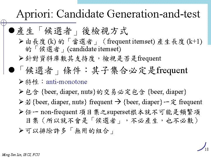
有意義程度Interestingness Measure: Correlations l play basketball eat cereal [40%, 66. 7%] 誤導！ Ø The overall percentage of students eating cereal is 75% which is higher than 66. 7%. l play basketball not eat cereal [20%, 33. 3%] 更精準, 雖然 support and confidence 較低 l 度量相依性/相關事件: lift Basketball Not basketball Sum (row) Cereal 2000 1750 3750 Not cereal 1000 250 1250 Sum(col. ) 3000 2000 52 Ming-Yen Lin, IECS, FCU

關聯規則的延伸與應用 l Correlation, causality analysis & mining interesting rules l Maxpatterns and frequent closed itemsets l Constraint-based mining l Sequential patterns l Association-based classification l Computing iceberg cubes 53 Ming-Yen Lin, IECS, FCU

l 最大樣式(max-patterns)與封閉樣式(closed patterns) Ø精簡的表示方式 l 多維度、多層次頻繁樣式 l 有意義程度(Interestingness): correlation and causality 54 Ming-Yen Lin, IECS, FCU

最大樣式Max-patterns l Frequent pattern {a 1, …, a 100} (1001) + (1002) + … + (110000) = 2100 -1 = 1. 27*1030 frequent subpatterns! l 最大樣式 Max-pattern: 沒有「真」(proper) super pattern的樣式 (PS: frequent) ØBCDE, ACD are max-patterns ØBCD is not a max-pattern m. s. =2 Tid 10 20 30 Items A, B, C, D, E, A, C, D, F 55 Ming-Yen Lin, IECS, FCU

Note on ARs l Many applications outside market basket data analysis ØPrediction (telecom switch failure) ØWeb usage mining l Many different types of association rules ØTemporal ØSpatial ØCausal 57 Ming-Yen Lin, IECS, FCU

Lex. Miner l Ming-Yen Lin and Suh-Yin Lee, "A Fast Lexicographic Algorithm for Association Rule Mining in Web Applications, " Proceedings of the ICDCS Workshop on Knowledge Discovery and Data Mining in the World-Wide Web (ICDCS 00), Taipei, Taiwan, R. O. C. , pp. F 7 -F 14, 2000. 58 Ming-Yen Lin, IECS, FCU

Apriori use Hash Tree to stored Candidates l Excess Comparison, Eg. T 1 = {1, 2, 3, 4, 5, 6} l Duplicate Counting Avoidance, Eg. T 2 = {1, 3, 4, 200, 401, 403} l Large Storage Requirement l High Splitting Cost : interior d=1 root 0 : leaf 1 d=2 2 d=3 Ming-Yen Lin, IECS, FCU (1, 2, 83) (1, 2, 95) (1, 2, 96) 3 2 3. . . : empty leaf (2, 3, 4) (2, 3, 5) (1, 3, 4) (1, 3, 9) (1, 403) (200, 401, 555) (198, 201, 203) (198, 400, 555) hash function = x MOD 199, size of each leaf = 5, d = depth . . . 59

Lex. Tree: Lexicographically Ordered Tree l Intrinsic Property: Lexicographic Order Ø Items in each transaction, eg. {7, 11, 20, 29, 37} Ø k-itemsets, eg. (1, 3, 4) < (1, 3, 10) < (1, 4, 10) l Storing itemsets: by lexicographic order l Lex. Tree: compact, hierarchical tree Ø candidate Lex. Tree: efficient, redundant-free support counting Ø frequent Lex. Tree: effective candidate generation l Lex. Miner Algorithm 60 Ming-Yen Lin, IECS, FCU

Lex. Tree Structure Item_ID Internal node: next Leaf node: sibling Item_ID support sibling Root 1 3 4 # 10 4 7 11 7 10 11 11 15 15 7 10 11 11 20 20 10 15 20 # # # # 4 3 10 # 11 10 # # 7 4 # # : support # # : null link (1, 3, 4), (1, 3, 10), (1, 3, 11), (1, 4, 10), (1, 4, 11), (1, 4, 15), (1, 10, 15), (3, 4, 7), (3, 4, 10), (3, 4, 11), (3, 7, 20), (3, 11, 20), (4, 7, 10), (4, 10, 15), (7, 11, 20) 61 Ming-Yen Lin, IECS, FCU

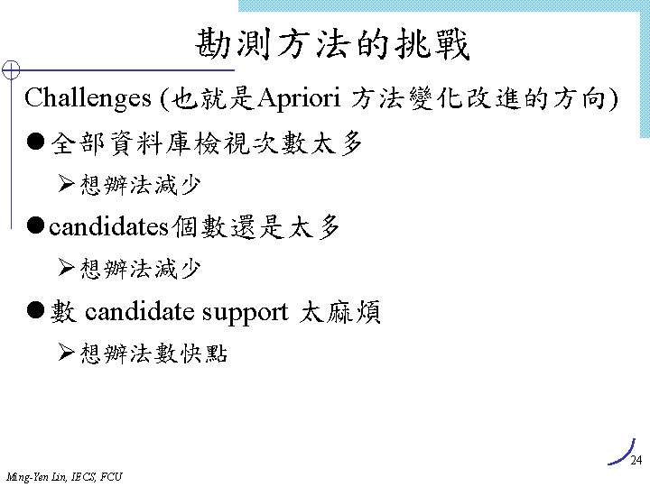
Lex. Tree Construction (1) Insert candidate (1, 3, 4) Root Last[1] 1 (2) Insert candidate (1, 3, 10) Root Last[1] 1 Last[2] 3 Last[3] 04 (3) Insert candidate (1, 3, 11) Root (4) Insert candidate (1, 4, 10) Root Last[1] 1 Last[2] 3 3 Last[3] 04 10 0 11 0 0 4 10 0 11 0 4 Last[2] 10 Last[3] 0 Insert candidates (1, 3, 4), (1, 3, 10), (1, 3, 11), (1, 4, 10) Ming-Yen Lin, IECS, FCU 62

Lex. Tree Construction (Cont. ) (5) Insert candidate (1, 10, 15) after (1, 4, 11), (1, 4, 15) inserted Root Last[1] 1 0 10 4 3 4 10 0 11 0 15 0 Last[2] Last[3] (6) Insert candidate (3, 4, 7) Root 3 Last[1] 10 4 Last[2] 15 7 Last[3] 1 4 3 0 4 10 0 11 0 15 0 0 0 63 Ming-Yen Lin, IECS, FCU

Notations l D : The database of transactions l T : A transaction, T={x 1, x 2, …, xp, …, xm} x 1, x 2, …, xk : Items l minsup : The minimum support specified by the user l X : k-itemset, X=(x 1, x 2, …, xk) l X. support : The support of itemset X l l Ck : The set of candidate k-itemsets Lk : The set of frequent k-itemsets Ck : The candidate k-itemset Lex. Tree Lk : The frequent k-itemset Lex. Tree 64 Ming-Yen Lin, IECS, FCU

Algorithm Lex. Miner N Find L 1 Build frequent Lk-1 from Lk-1 L 1 Generate Ck from Lk-1 Y Store Ck in candidate Ck Find L 2 T D, Find_and_increment(T , Ck) k=3 N Lk-1 Y Lk= {X Ck | X. support minsup} k++ Answer = k LFCU k Ming-Yen Lin, IECS, 65

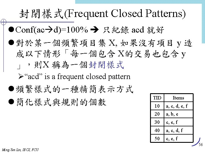
Algorithm Find_and_Increment Internal node item[tp] ? cp. ID Y tp advanced < Find_and_Increment(tp, cp) Find_and_Increment(tp+1, cp. sibling) Find_and_Increment(tp+1, cp. next) = > cp advanced Find_and_Increment(tp, cp) cp leaf < N Leaf node advance tp item[tp] ? cp. ID = > cp. support++ Advance tp and cp advance cp while (not end_of_list) and (cp null) Ming-Yen Lin, IECS, FCU 66

Example 1: #Comparison Minimized q At pass 3, T 1={7, 11, 20, 29, 37} Intrinsically ordered 3 -itemsets in T 1 { 7, 11} {20, 29, 37} { 7, 20} {29, 37} { 7, 29} {37} {11, 20} {29, 37} {11, 29} {37} {20, 29} {37} 7 11 (20, 29, 37) 20 (29, 37) 29 (37) 11 20 (29, 37) 29 (37) 20 29 (37) Root Na Nb 1 4 3 4 # 10 # 11 # Ming-Yen Lin, IECS, FCU 10 # 11 # 15 # 10 4 15 7 # # 7 10 # 11 # 20 # Candidate 3 -itemset Lex. Tree, C 3 Nd Nc 4 11 7 10 11 20 10 15 20 3 # # # 7 # Ne Nf 67

Example 2: Fast Support Counting q At pass 3, T 2={3, 4, 7, 10, 11} Intrinsically ordered 3 -itemsets in T 2 3 x 4 x (7, 10, 11) x 7 x (10, 11) x 10 x (11) 4 x 7 x (10, 11) x 10 x (11) 7 x 10 x (11) Root Na Nb 1 4 3 4 # 10 # 11 # 15 # 3 10 4 15 7 # # Nj # Nk 11 Nd 7 Nh Ni 11 7 10 11 11 20 20 10 15 20 # # 4 7 Ng 10 Nc # # # Ne Nf Nl Candidate 3 -itemset Lex. Tree, C 3 68 Ming-Yen Lin, IECS, FCU

Efficient Candidate Generation l Common prefixed Lk-1 : linked by sibling l Join: Ck = Lk-1, then insert into Ck select p[1], p[2], …, p[k-1], q[k-1] from Lk-1 p, Lk-1 q where p[1]=q[1], …, p[k-2] = q[k-2], p[k-1] < q[k-1] ; l Prune: candidate itemset having any subset that is not in Lk-1 Ø Searching in Lk-1 : similar technique for find_and_increment Ming-Yen Lin, IECS, FCU 69

FP-growth l J. Han, J. Pei, and Y. Yin: “Mining frequent patterns without candidate generation”. In Proc. ACM-SIGMOD’ 2000, pp. 1 -12, Dallas, TX, May 2000. l Compress DB into a tree (FP-tree) l Find frequent itemsets in FP-tree 70 Ming-Yen Lin, IECS, FCU

Construction of FP-tree from a Transaction Database TID 100 200 300 400 500 Items bought (ordered) frequent items {f, a, c, d, g, i, m, p} {f, c, a, m, p} {a, b, c, f, l, m, o} {f, c, a, b, m} {b, f, h, j, o, w} {f, b} {b, c, k, s, p} {c, b, p} {a, f, c, e, l, p, m, n} {f, c, a, m, p} 1. Scan DB once, find frequent 1 -itemset (single item pattern) 2. Order frequent items in frequency descending order 3. Scan DB again, construct FP-tree Ming-Yen Lin, IECS, FCU min_support = 0. 5 {} Header Table Item frequency head f 4 c 4 a 3 b 3 m 3 p 3 f: 4 c: 3 c: 1 b: 1 a: 3 b: 1 p: 1 m: 2 b: 1 p: 2 m: 1 71

Mining Frequent Patterns with FP-trees l Idea: Frequent pattern growth Ø Recursively grow frequent patterns by pattern and database partition l Method Ø For each frequent item, construct its conditional patternbase, and then its conditional FP-tree Ø Repeat the process on each newly created conditional FPtree Ø Until the resulting FP-tree is empty, or it contains only one path —single path will generate all the combinations of its sub-paths, each of which is a frequent pattern 72 Ming-Yen Lin, IECS, FCU

From FP-tree to Conditional Pattern-Base l Starting at the frequent item header table in the FP-tree l Traverse the FP-tree by following the link of each frequent item p l Accumulate all of transformed prefix paths of item p to form p’s conditional pattern base {} Header Table Item frequency head f 4 c 4 a 3 b 3 m 3 p 3 Ming-Yen Lin, IECS, FCU Conditional pattern bases f: 4 c: 3 c: 1 b: 1 a: 3 b: 1 p: 1 m: 2 b: 1 p: 2 m: 1 item cond. pattern base c f: 3 a fc: 3 b fca: 1, f: 1, c: 1 m fca: 2, fcab: 1 p fcam: 2, cb: 1 73

Transformed Prefix Paths l Derive the transformed prefix paths of item p Ø For each item p in the tree, collect p’s prefix path with count = p’s frequency Ø Why only prefix path? Why this count? Complete? {} Header Table Item frequency head f 4 c 4 a 3 b 3 m 3 p 3 f: 4 c: 3 b: 1 a: 3 m: 2 p: 2 Ming-Yen Lin, IECS, FCU c: 1 b: 1 p: 1 b: 1 m: 1 Conditional pattern bases item cond. pattern base c f: 3 a fc: 3 b fca: 1, f: 1, c: 1 m fca: 2, fcab: 1 p fcam: 2, cb: 1 74

From Conditional Pattern-Bases to Conditional FP-trees l For each pattern-base Ø Accumulate the count for each item in the base Ø Construct the FP-tree for the frequent items of the pattern base Header Table Item frequency head f 4 c 4 a 3 b 3 m 3 p 3 m-conditional pattern base: fca: 2, fcab: 1 {} f: 4 c: 3 c: 1 b: 1 a: 3 b: 1 p: 1 {} f: 3 m: 2 b: 1 c: 3 p: 2 m: 1 a: 3 All frequent patterns relate to m m, fm, cm, am, fcm, fam, cam, fcam m-conditional FP-tree Ming-Yen Lin, IECS, FCU 75

Recursion: Mining Each Conditional FP-tree Until … {} {} Cond. pattern base of “am”: (fc: 3) c: 3 f: 3 c: 3 a: 3 f: 3 am-conditional FP-tree Cond. pattern base of “cm”: (f: 3) {} f: 3 m-conditional FP-tree cm-conditional FP-tree {} Cond. pattern base of “cam”: (f: 3) f: 3 cam-conditional FP-tree 76 Ming-Yen Lin, IECS, FCU

A Special Case: Single FP-tree Path l Suppose a (conditional) FP-tree T has a single path P l The complete set of frequent patterns of T can be generated by enumeration of all the combinations of the sub-paths of P {} f: 3 c: 3 a: 3 All frequent patterns concerning m m, fm, cm, am, fcm, fam, cam, fcam m-conditional FP-tree 77 Ming-Yen Lin, IECS, FCU

A More General (Special) Case: Single Prefix Path in FP-tree l Suppose a (conditional) FP-tree T has a shared single prefix-path P l Mining can be decomposed into two parts {} a 1: n 1 Ø Reduction of the single prefix path into one node Ø Concatenation of the mining results of the two parts a 2: n 2 a 3: n 3 b 1: m 1 r 1 {} C 1: k 1 C 2: k 2 Ming-Yen Lin, IECS, FCU C 3: k 3 r 1 = a 1: n 1 a 2: n 2 a 3: n 3 + b 1: m 1 C 2: k 2 C 1: k 1 C 3: k 3 78