Association Analysis 3 Alternative Methods for Frequent Itemset
- Slides: 32

Association Analysis (3)

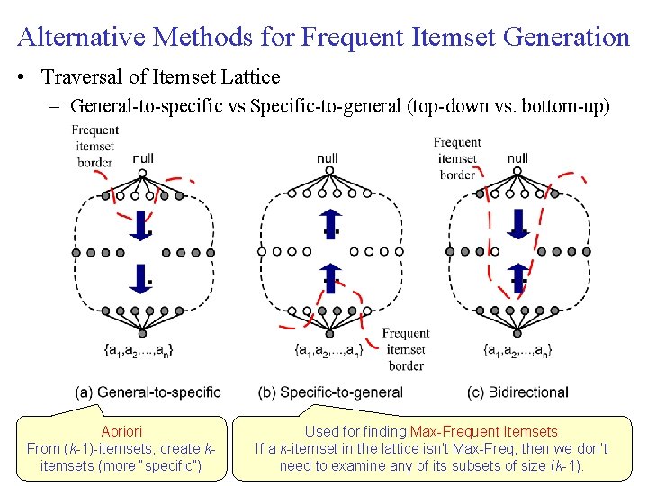
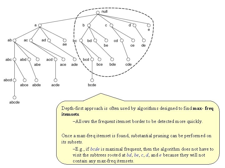
Alternative Methods for Frequent Itemset Generation • Traversal of Itemset Lattice – General to specific vs Specific to general (top down vs. bottom up) Apriori From (k 1) itemsets, create k itemsets (more “specific”) Used for finding Max Frequent Itemsets If a k itemset in the lattice isn’t Max Freq, then we don’t need to examine any of its subsets of size (k 1).

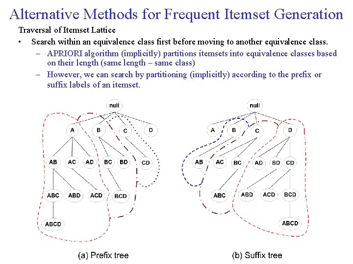
Alternative Methods for Frequent Itemset Generation Traversal of Itemset Lattice • Search within an equivalence class first before moving to another equivalence class. – APRIORI algorithm (implicitly) partitions itemsets into equivalence classes based on their length (same length – same class) – However, we can search by partitioning (implicitly) according to the prefix or suffix labels of an itemset.

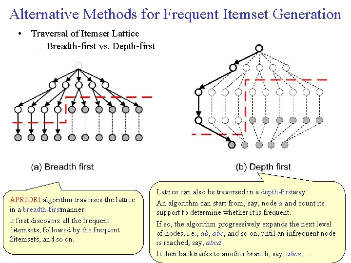
Alternative Methods for Frequent Itemset Generation • Traversal of Itemset Lattice – Breadth first vs. Depth first APRIORI algorithm traverses the lattice in a breadth firstmanner. It first discovers all the frequent 1 itemsets, followed by the frequent 2 itemsets, and so on. Lattice can also be traversed in a depth firstway. An algorithm can start from, say, node a and count its support to determine whether it is frequent. If so, the algorithm progressively expands the next level of nodes, i. e. , abc, and so on, until an infrequent node is reached, say, abcd. It then backtracks to another branch, say, abce, …

Depth first approach is often used by algorithms designed to find max freq itemsets. –Allows the frequent itemset border to be detected more quickly. Once a max freq itemset is found, substantial pruning can be performed on its subsets. –E. g. , if bcde is maximal frequent, then the algorithm does not have to visit the subtrees rooted at bd, be, c, d, and e because they will not contain any max freq itemsets.

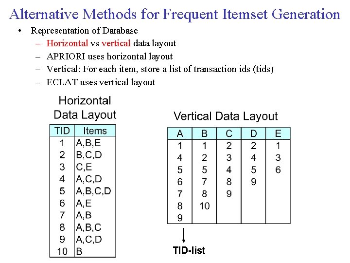
Alternative Methods for Frequent Itemset Generation • Representation of Database – Horizontal vs vertical data layout – APRIORI uses horizontal layout – Vertical: For each item, store a list of transaction ids (tids) – ECLAT uses vertical layout TID-list

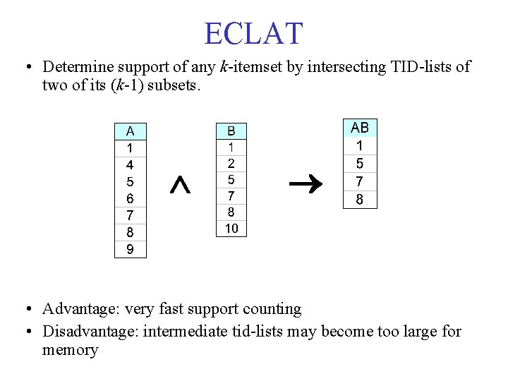
ECLAT • Determine support of any k itemset by intersecting TID lists of two of its (k 1) subsets. • Advantage: very fast support counting • Disadvantage: intermediate tid lists may become too large for memory

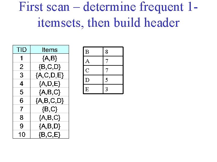
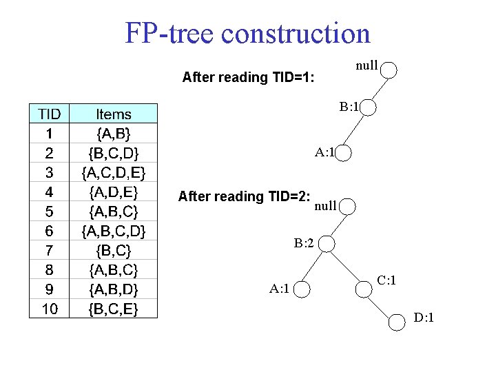
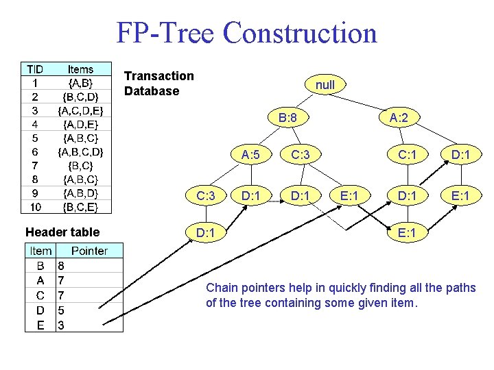
FP Tree/FP Growth Algorithm • Use a compressed representation of the database using an FP tree • Once an FP tree has been constructed, it uses a recursive divide and conquer approach to mine the frequent itemsets. Building the FP Tree 1. Scan data to determine the support count of each item. Infrequent items are discarded, while the frequent items are sorted in decreasing support counts. 2. Make a second pass over the data to construct the FP tree. As the transactions are read, before being processed, their items are sorted according to the above order.

First scan – determine frequent 1 itemsets, then build header B 8 A 7 C 7 D 5 E 3

FP tree construction null After reading TID=1: B: 1 After reading TID=2: null B: 2 A: 1 C: 1 D: 1

FP Tree Construction Transaction Database null B: 8 C: 3 Header table D: 1 A: 5 C: 3 D: 1 A: 2 E: 1 C: 1 D: 1 E: 1 Chain pointers help in quickly finding all the paths of the tree containing some given item.

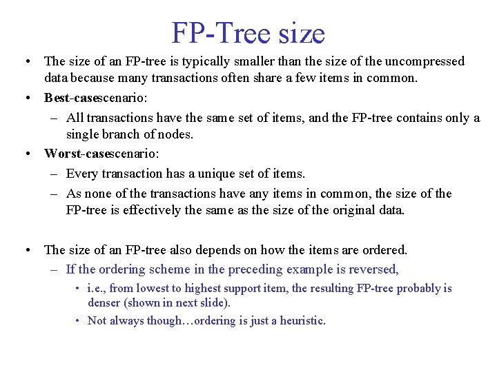
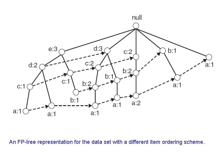
FP Tree size • The size of an FP tree is typically smaller than the size of the uncompressed data because many transactions often share a few items in common. • Best casescenario: – All transactions have the same set of items, and the FP tree contains only a single branch of nodes. • Worst casescenario: – Every transaction has a unique set of items. – As none of the transactions have any items in common, the size of the FP tree is effectively the same as the size of the original data. • The size of an FP tree also depends on how the items are ordered. – If the ordering scheme in the preceding example is reversed, • i. e. , from lowest to highest support item, the resulting FP tree probably is denser (shown in next slide). • Not always though…ordering is just a heuristic.

An FP tree representation for the data set with a different item ordering scheme.

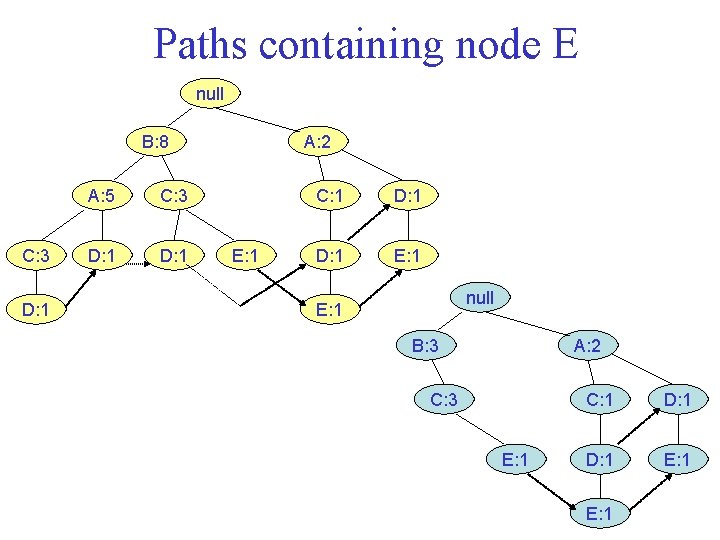
FP Growth (I) • FP growth generates frequentitemsets from an FP tree by exploring the tree in a bottom up fashion. • Given the example tree, the algorithm looks for frequent itemsets ending in E first, followed by D, C, A, and finally, B. • Since every transaction is mapped onto a path in the FP tree, we can derive the frequent itemsets ending with a particular item, say, E, by examining only the paths containing node E. • These paths can be accessed rapidly using the pointers associated with node E.

Paths containing node E null B: 8 C: 3 D: 1 A: 5 C: 3 D: 1 A: 2 E: 1 C: 1 D: 1 E: 1 null E: 1 B: 3 A: 2 C: 3 E: 1 C: 1 D: 1 E: 1

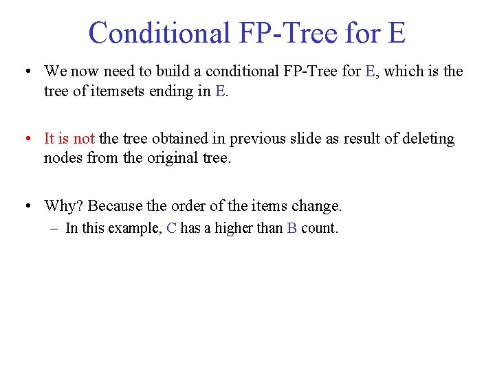
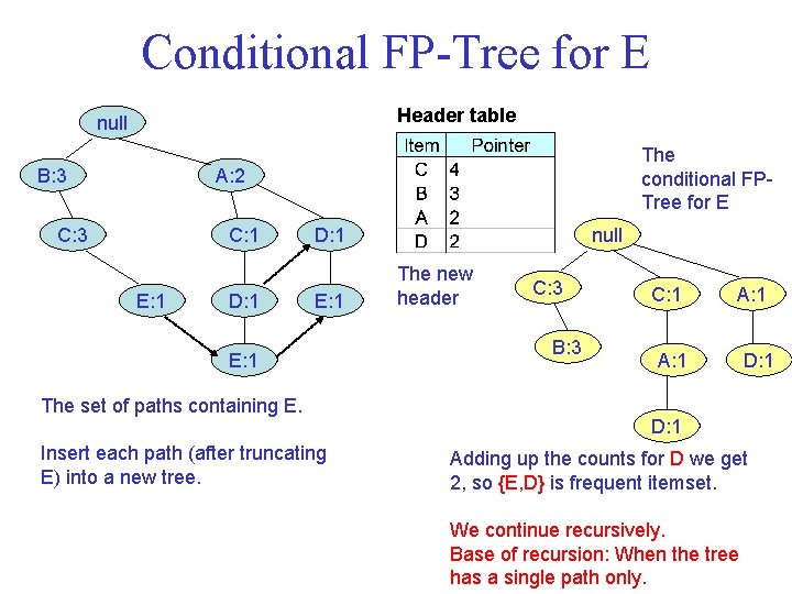
Conditional FP Tree for E • We now need to build a conditional FP Tree for E, which is the tree of itemsets ending in E. • It is not the tree obtained in previous slide as result of deleting nodes from the original tree. • Why? Because the order of the items change. – In this example, C has a higher than B count.

Conditional FP Tree for E Header table null B: 3 The conditional FP Tree for E A: 2 C: 3 C: 1 E: 1 D: 1 null D: 1 E: 1 The set of paths containing E. Insert each path (after truncating E) into a new tree. The new header C: 3 B: 3 C: 1 A: 1 D: 1 Adding up the counts for D we get 2, so {E, D} is frequent itemset. We continue recursively. Base of recursion: When the tree has a single path only.

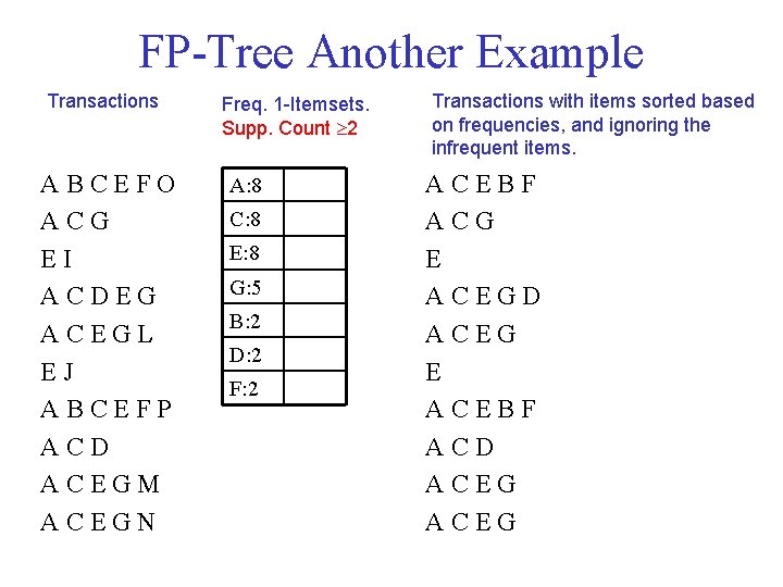
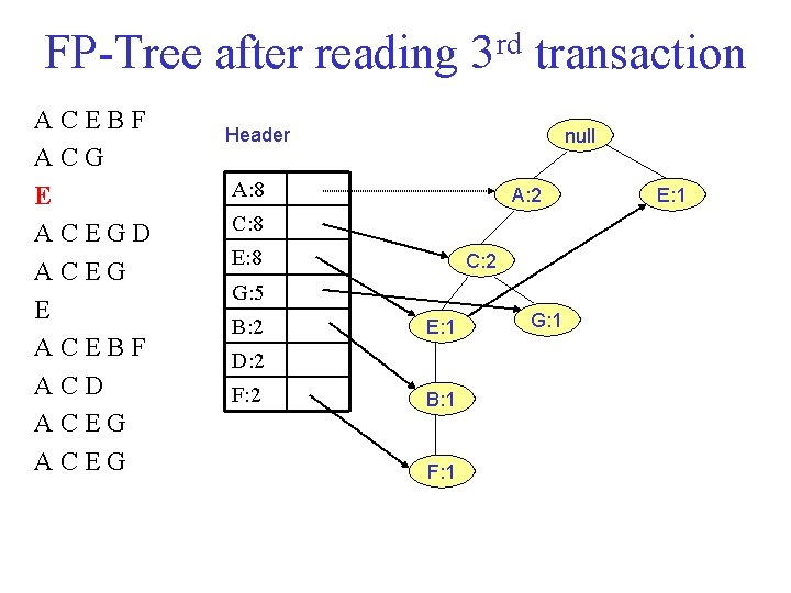
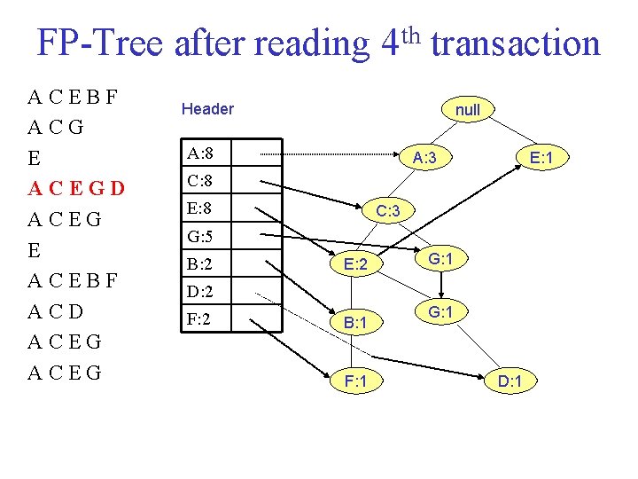
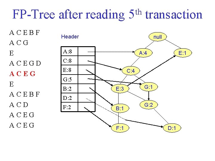
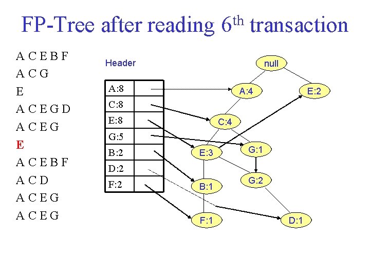
FP Tree Another Example Transactions ABCEFO ACG EI ACDEG ACEGL EJ ABCEFP ACD ACEGM ACEGN Freq. 1 Itemsets. Supp. Count 2 A: 8 C: 8 E: 8 G: 5 B: 2 D: 2 F: 2 Transactions with items sorted based on frequencies, and ignoring the infrequent items. ACEBF ACG E ACEGD ACEG E ACEBF ACD ACEG

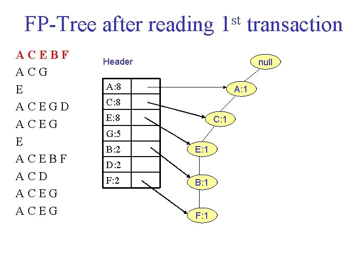
FP Tree after reading 1 st transaction ACEBF ACG E ACEGD ACEG E ACEBF ACD ACEG Header null A: 8 A: 1 C: 8 E: 8 C: 1 G: 5 B: 2 E: 1 D: 2 F: 2 B: 1 F: 1

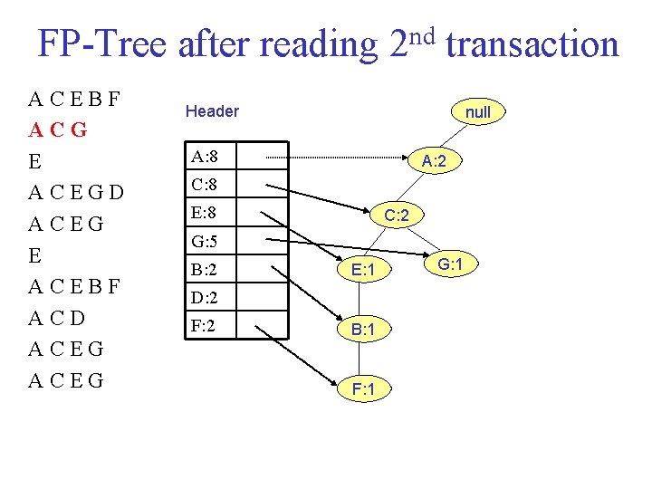
FP Tree after reading 2 nd transaction ACEBF ACG E ACEGD ACEG E ACEBF ACD ACEG Header null A: 8 A: 2 C: 8 E: 8 C: 2 G: 5 B: 2 E: 1 D: 2 F: 2 B: 1 F: 1 G: 1

FP Tree after reading 3 rd transaction ACEBF ACG E ACEGD ACEG E ACEBF ACD ACEG Header null A: 8 A: 2 C: 8 E: 8 C: 2 G: 5 B: 2 E: 1 D: 2 F: 2 B: 1 F: 1 G: 1 E: 1

FP Tree after reading 4 th transaction ACEBF ACG E ACEGD ACEG E ACEBF ACD ACEG Header null A: 8 A: 3 E: 1 C: 8 E: 8 C: 3 G: 5 B: 2 E: 2 G: 1 D: 2 F: 2 B: 1 F: 1 G: 1 D: 1

FP Tree after reading 5 th transaction ACEBF ACG E ACEGD ACEG E ACEBF ACD ACEG Header null A: 8 A: 4 E: 1 C: 8 E: 8 C: 4 G: 5 B: 2 E: 3 G: 1 D: 2 F: 2 B: 1 F: 1 G: 2 D: 1

FP Tree after reading 6 th transaction ACEBF ACG E ACEGD ACEG E ACEBF ACD ACEG Header null A: 8 A: 4 E: 2 C: 8 E: 8 C: 4 G: 5 B: 2 E: 3 G: 1 D: 2 F: 2 B: 1 F: 1 G: 2 D: 1

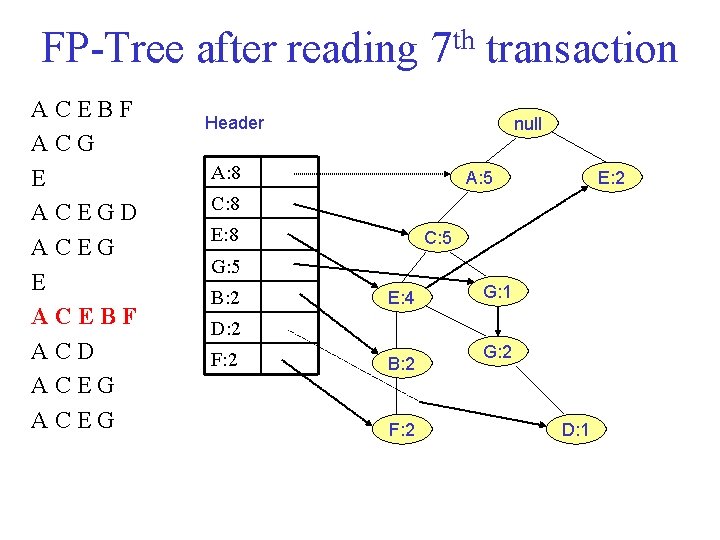
FP Tree after reading 7 th transaction ACEBF ACG E ACEGD ACEG E ACEBF ACD ACEG Header null A: 8 A: 5 E: 2 C: 8 E: 8 C: 5 G: 5 B: 2 E: 4 G: 1 D: 2 F: 2 B: 2 F: 2 G: 2 D: 1

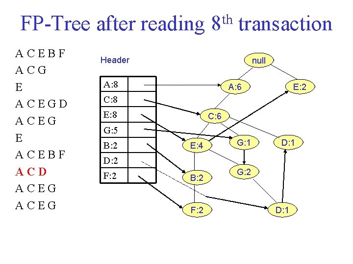
FP Tree after reading 8 th transaction ACEBF ACG E ACEGD ACEG E ACEBF ACD ACEG Header null A: 8 A: 6 E: 2 C: 8 E: 8 C: 6 G: 5 B: 2 E: 4 G: 1 D: 2 F: 2 B: 2 F: 2 G: 2 D: 1

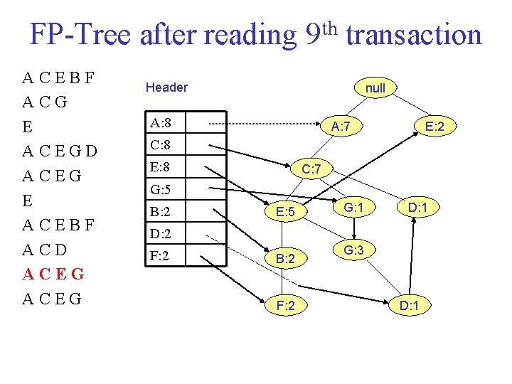
FP Tree after reading 9 th transaction ACEBF ACG E ACEGD ACEG E ACEBF ACD ACEG Header null A: 8 A: 7 E: 2 C: 8 E: 8 C: 7 G: 5 B: 2 E: 5 G: 1 D: 2 F: 2 B: 2 F: 2 G: 3 D: 1

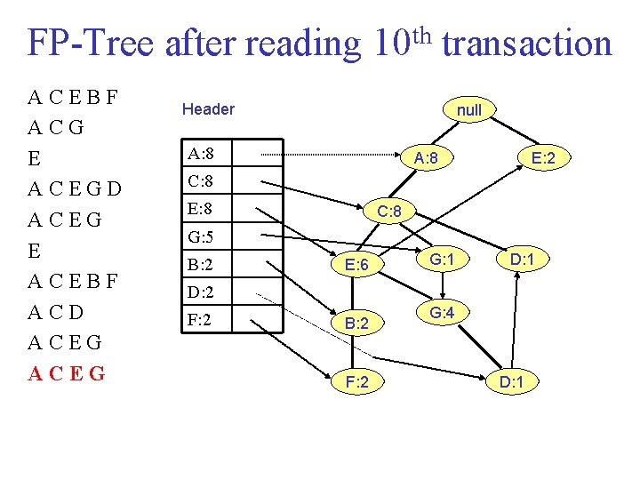
FP Tree after reading 10 th transaction ACEBF ACG E ACEGD ACEG E ACEBF ACD ACEG Header null A: 8 E: 2 C: 8 E: 8 C: 8 G: 5 B: 2 E: 6 G: 1 D: 2 F: 2 B: 2 F: 2 G: 4 D: 1

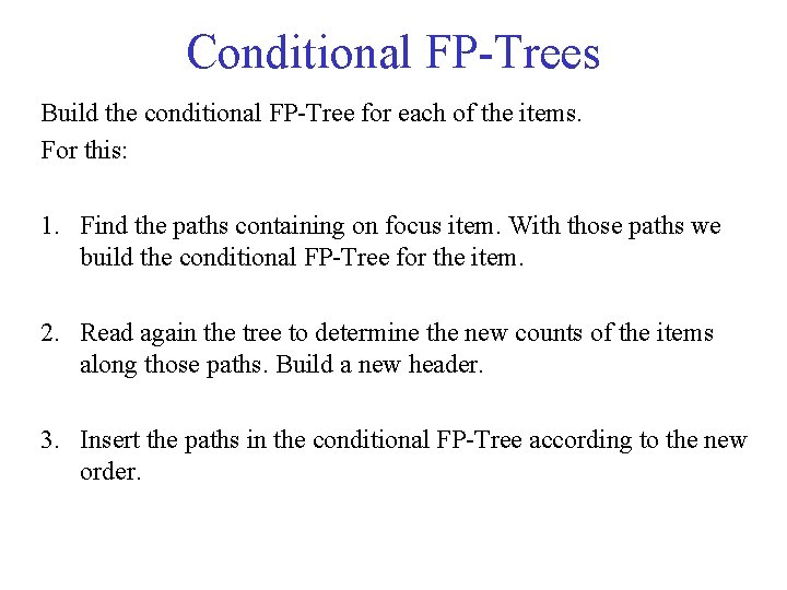
Conditional FP Trees Build the conditional FP Tree for each of the items. For this: 1. Find the paths containing on focus item. With those paths we build the conditional FP Tree for the item. 2. Read again the tree to determine the new counts of the items along those paths. Build a new header. 3. Insert the paths in the conditional FP Tree according to the new order.

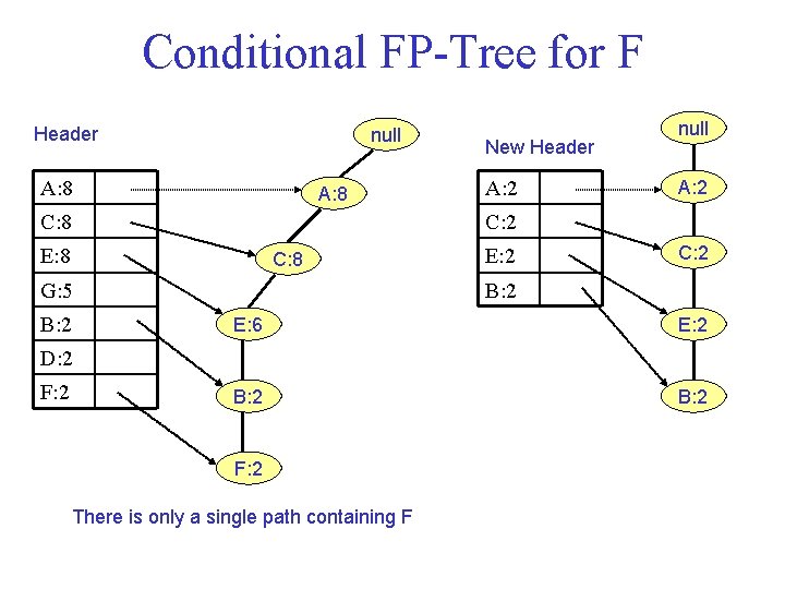
Conditional FP Tree for F Header null A: 8 A: 2 C: 8 E: 8 C: 8 E: 2 C: 2 B: 2 G: 5 B: 2 New Header null E: 6 E: 2 B: 2 D: 2 F: 2 There is only a single path containing F

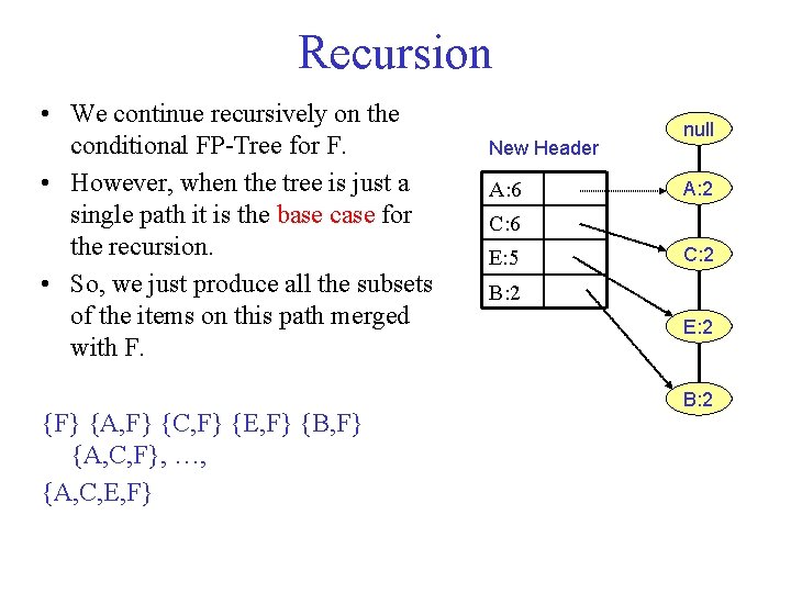
Recursion • We continue recursively on the conditional FP Tree for F. • However, when the tree is just a single path it is the base case for the recursion. • So, we just produce all the subsets of the items on this path merged with F. {F} {A, F} {C, F} {E, F} {B, F} {A, C, F}, …, {A, C, E, F} New Header A: 6 null A: 2 C: 6 E: 5 C: 2 B: 2 E: 2 B: 2

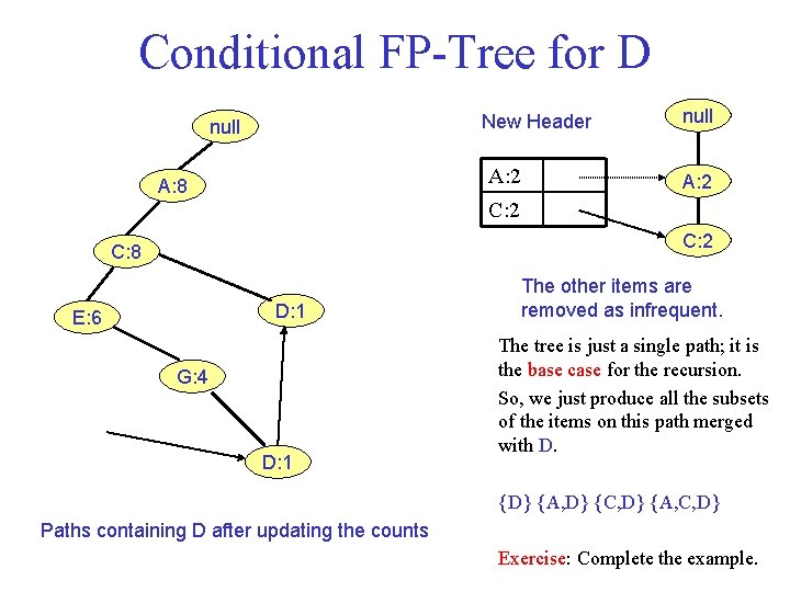
Conditional FP Tree for D New Header null A: 2 A: 8 null A: 2 C: 8 D: 1 E: 6 G: 4 D: 1 The other items are removed as infrequent. The tree is just a single path; it is the base case for the recursion. So, we just produce all the subsets of the items on this path merged with D. {D} {A, D} {C, D} {A, C, D} Paths containing D after updating the counts Exercise: Complete the example.