Still More StreamMining Frequent Itemsets Elephants and Troops

Still More Stream-Mining Frequent Itemsets Elephants and Troops Exponentially Decaying Windows 1

Counting Items u. Problem: given a stream, which items appear more than s times in the window? u. Possible solution: think of the stream of baskets as one binary stream per item. w 1 = item present; 0 = not present. w Use DGIM to estimate counts of 1’s for all items. 2

Extensions u In principle, you could count frequent pairs or even larger sets the same way. w One stream per itemset. u Drawbacks: 1. Only approximate. 2. Number of itemsets is way too big. 3

Approaches 1. “Elephants and troops”: a heuristic way to converge on unusually strongly connected itemsets. 2. Exponentially decaying windows: a heuristic for selecting likely frequent itemsets. 4

Elephants and Troops u. When Sergey Brin wasn’t worrying about Google, he tried the following experiment. u. Goal: find unusually correlated sets of words. w “High Correlation ” = frequency of occurrence of set >> product of frequency of members. 5

Experimental Setup u. The data was an early Google crawl of the Stanford Web. u. Each night, the data would be streamed to a process that counted a preselected collection of itemsets. w If {a, b, c} is selected, count {a, b, c}, {a}, {b}, and {c}. w “Correlation” = n 2 * #abc/(#a * #b * #c). • n = number of pages. 6

After Each Night’s Processing. . . 1. Find the most correlated sets counted. 2. Construct a new collection of itemsets to count the next night. w All the most correlated sets (“winners ”). w Pairs of a word in some winner and a random word. w Winners combined in various ways. w Some random pairs. 7

After a Week. . . u. The pair {“elephants”, “troops”} came up as the big winner. u. Why? It turns out that Stanford students were playing a Punic-War simulation game internationally, where moves were sent by Web pages. 8

Mining Streams Vs. Mining DB’s (New Topic) u. Unlike mining databases, mining streams doesn’t have a fixed answer. u. We’re really mining in the “Stat” point of view, e. g. , “Which itemsets are frequent in the underlying model that generates the stream? ” 9

Stationarity u Two different assumptions make a big difference. 1. Is the model stationary ? u I. e. , are the same statistics used throughout all time to generate the stream? 2. Or does the frequency of generating given items or itemsets change over time? 10

Some Options for Frequent Itemsets u We could: 1. Run periodic experiments, like E&T. u Like SON --- itemset is a candidate if it is found frequent on any “day. ” u Good for stationary statistics. 2. Frame the problem as finding all frequent itemsets in an “exponentially decaying window. ” u Good for nonstationary statistics. 11

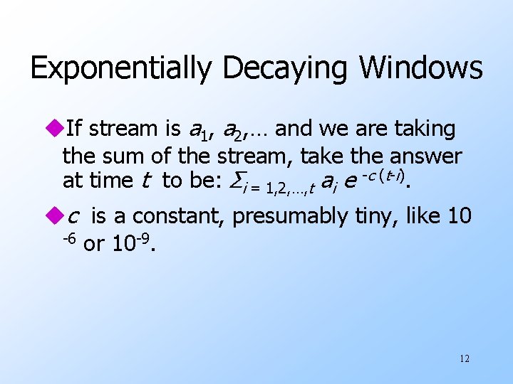
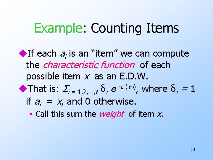
Exponentially Decaying Windows u. If stream is a 1, a 2, … and we are taking the sum of the stream, take the answer at time t to be: Σi = 1, 2, …, t ai e -c (t-i). uc is a constant, presumably tiny, like 10 -6 or 10 -9. 12

Example: Counting Items u. If each ai is an “item” we can compute the characteristic function of each possible item x as an E. D. W. u. That is: Σi = 1, 2, …, t δi e -c (t-i), where δi = 1 if ai = x, and 0 otherwise. w Call this sum the weight of item x. 13

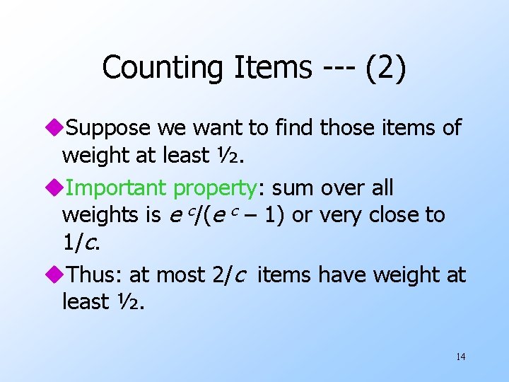
Counting Items --- (2) u. Suppose we want to find those items of weight at least ½. u. Important property: sum over all weights is e c/(e c – 1) or very close to 1/c. u. Thus: at most 2/c items have weight at least ½. 14

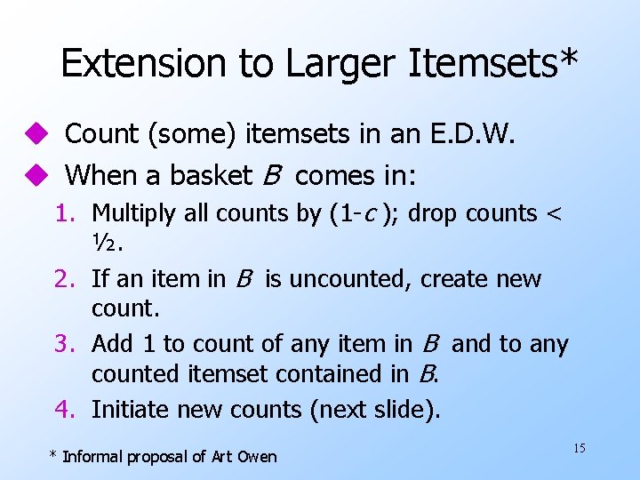
Extension to Larger Itemsets* u Count (some) itemsets in an E. D. W. u When a basket B comes in: 1. Multiply all counts by (1 -c ); drop counts < ½. 2. If an item in B is uncounted, create new count. 3. Add 1 to count of any item in B and to any counted itemset contained in B. 4. Initiate new counts (next slide). * Informal proposal of Art Owen 15

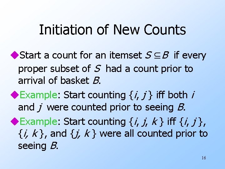
Initiation of New Counts u. Start a count for an itemset S ⊆B if every proper subset of S had a count prior to arrival of basket B. u. Example: Start counting {i, j } iff both i and j were counted prior to seeing B. u. Example: Start counting {i, j, k } iff {i, j }, {i, k }, and {j, k } were all counted prior to seeing B. 16

How Many Counts? u. Counts for single items = (2/c ) times the average number of items in a basket. u. Counts for larger itemsets = ? ? . But we are conservative about starting counts of large sets. w If we counted every set we saw, one basket of 20 items would initiate 1 M counts. 17