Clustering CSE 4309 Machine Learning Vassilis Athitsos Computer

Clustering CSE 4309 – Machine Learning Vassilis Athitsos Computer Science and Engineering Department University of Texas at Arlington 1

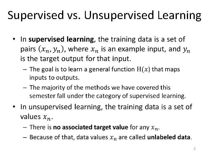
Supervised vs. Unsupervised Learning • 2

Supervised vs. Unsupervised Learning • The goal in supervised learning is regression or classification. • The goal in unsupervised learning is to discover hidden structure in the data. 3

Supervised vs. Unsupervised Learning • You may have heard of some methods that do different types of unsupervised learning. – PCA (principal component analysis): it learns how to represent highdimensional vectors using low-dimensional vectors. – SVD (singular value decomposition): it learns how to represent matrix data as dot products of low-dimensional vectors. An example of such matrix data is movie ratings by users (one row per user, one column per movie, most values left unspecified), where we can use SVD to build a model that predicts how much a specific user will like a specific movie. • We will cover some of these methods towards the end of the semester, as optional, non-graded material. 4

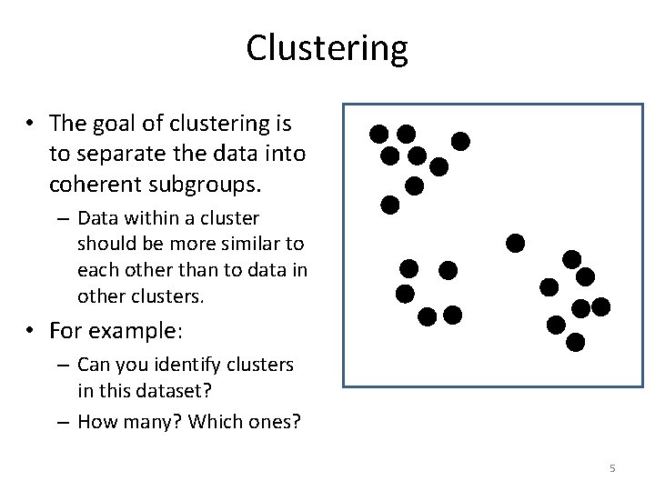
Clustering • The goal of clustering is to separate the data into coherent subgroups. – Data within a cluster should be more similar to each other than to data in other clusters. • For example: – Can you identify clusters in this dataset? – How many? Which ones? 5

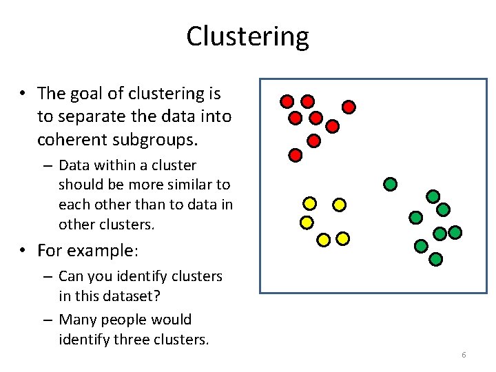
Clustering • The goal of clustering is to separate the data into coherent subgroups. – Data within a cluster should be more similar to each other than to data in other clusters. • For example: – Can you identify clusters in this dataset? – Many people would identify three clusters. 6

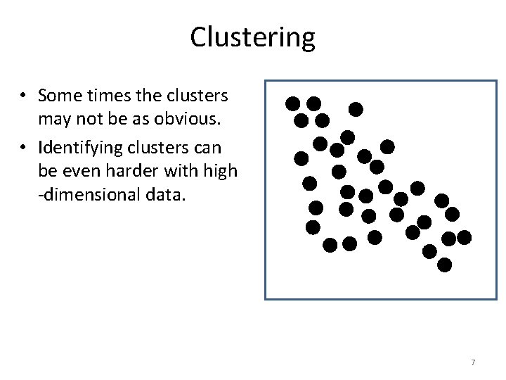
Clustering • Some times the clusters may not be as obvious. • Identifying clusters can be even harder with high -dimensional data. 7

Applications of Clustering • Finding subgroups of similar items is useful in many fields: – In biology, clustering is used to identify relationships between organisms, and to uncover possible evolutionary links. – In marketing, clustering is used to identify segments of the population that would be specific targets for specific products. – For anomaly detection, anomalous data can be identified as data that cannot be assigned to any of the "normal" clusters. – In search engines and recommender systems, clustering can be used to group similar items together. 8

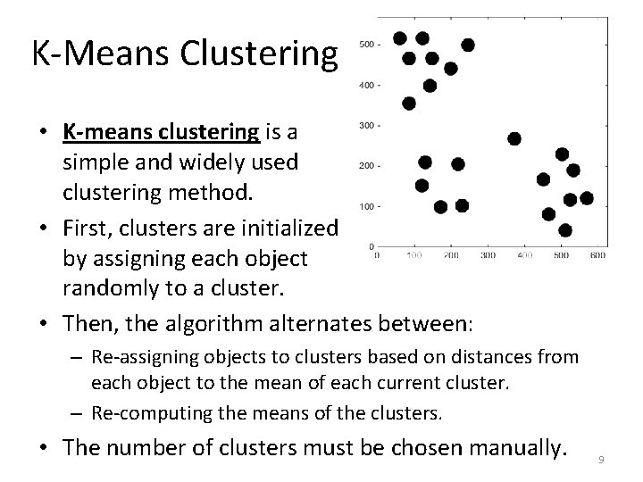
K-Means Clustering • K-means clustering is a simple and widely used clustering method. • First, clusters are initialized by assigning each object randomly to a cluster. • Then, the algorithm alternates between: – Re-assigning objects to clusters based on distances from each object to the mean of each current cluster. – Re-computing the means of the clusters. • The number of clusters must be chosen manually. 9

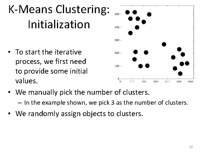
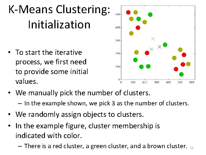
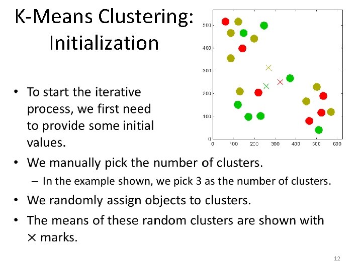
K-Means Clustering: Initialization • To start the iterative process, we first need to provide some initial values. • We manually pick the number of clusters. – In the example shown, we pick 3 as the number of clusters. • We randomly assign objects to clusters. 10

K-Means Clustering: Initialization • To start the iterative process, we first need to provide some initial values. • We manually pick the number of clusters. – In the example shown, we pick 3 as the number of clusters. • We randomly assign objects to clusters. • In the example figure, cluster membership is indicated with color. – There is a red cluster, a green cluster, and a brown cluster. 11

K-Means Clustering: Initialization • 12

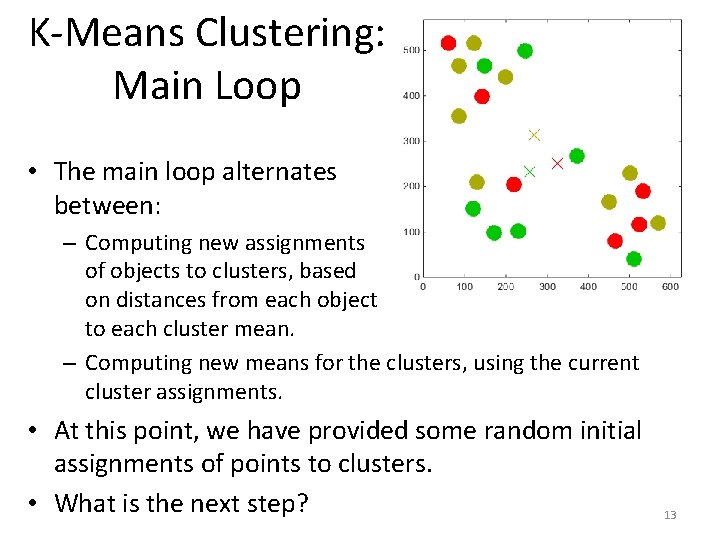
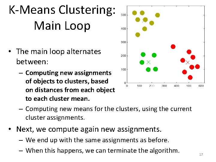
K-Means Clustering: Main Loop • The main loop alternates between: – Computing new assignments of objects to clusters, based on distances from each object to each cluster mean. – Computing new means for the clusters, using the current cluster assignments. • At this point, we have provided some random initial assignments of points to clusters. • What is the next step? 13

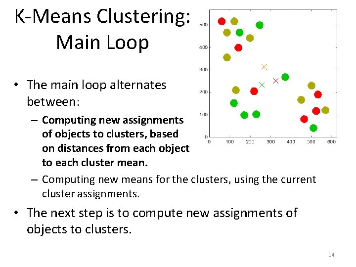
K-Means Clustering: Main Loop • The main loop alternates between: – Computing new assignments of objects to clusters, based on distances from each object to each cluster mean. – Computing new means for the clusters, using the current cluster assignments. • The next step is to compute new assignments of objects to clusters. 14

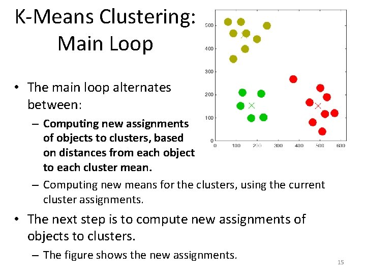
K-Means Clustering: Main Loop • The main loop alternates between: – Computing new assignments of objects to clusters, based on distances from each object to each cluster mean. – Computing new means for the clusters, using the current cluster assignments. • The next step is to compute new assignments of objects to clusters. – The figure shows the new assignments. 15

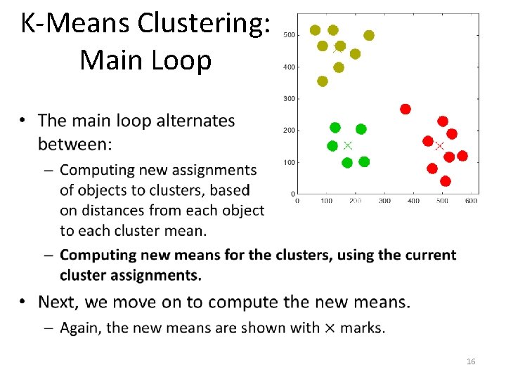
K-Means Clustering: Main Loop • 16

K-Means Clustering: Main Loop • The main loop alternates between: – Computing new assignments of objects to clusters, based on distances from each object to each cluster mean. – Computing new means for the clusters, using the current cluster assignments. • Next, we compute again new assignments. – We end up with the same assignments as before. – When this happens, we can terminate the algorithm. 17

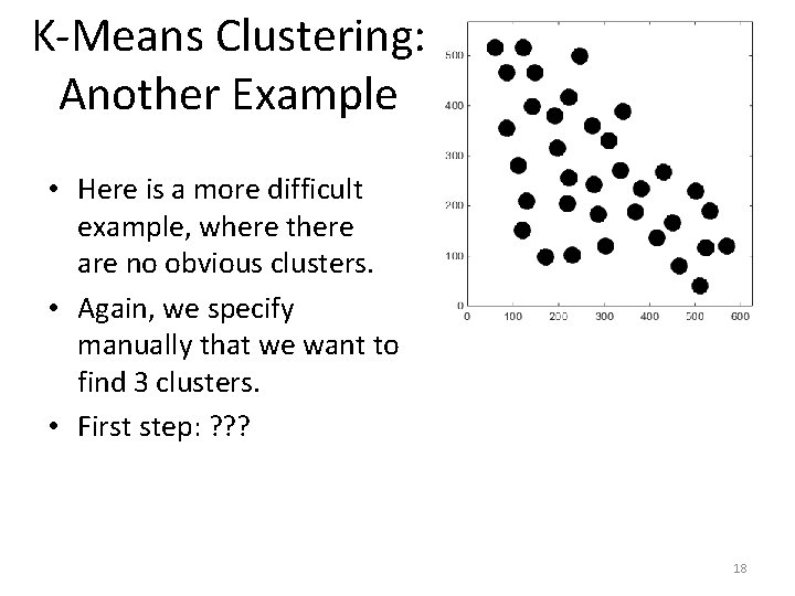
K-Means Clustering: Another Example • Here is a more difficult example, where there are no obvious clusters. • Again, we specify manually that we want to find 3 clusters. • First step: ? ? ? 18

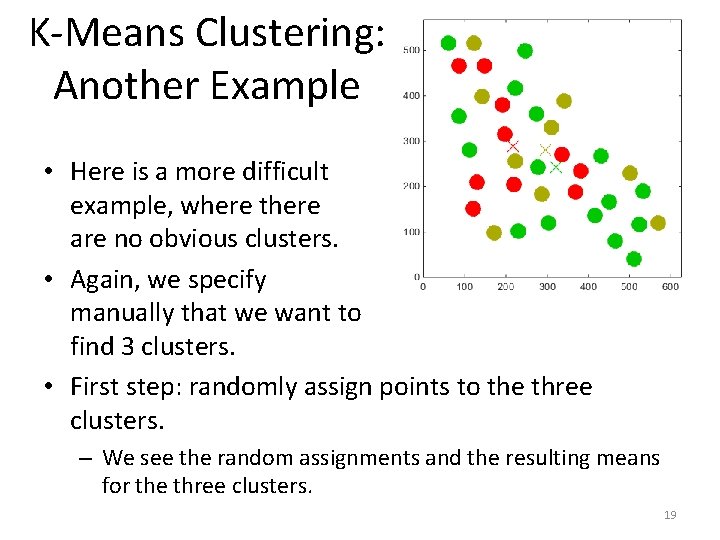
K-Means Clustering: Another Example • Here is a more difficult example, where there are no obvious clusters. • Again, we specify manually that we want to find 3 clusters. • First step: randomly assign points to the three clusters. – We see the random assignments and the resulting means for the three clusters. 19

K-Means Clustering: Another Example • Here is a more difficult example, where there are no obvious clusters. • Again, we specify manually that we want to find 3 clusters. • Main loop, iteration 1: recompute cluster assignments. 20

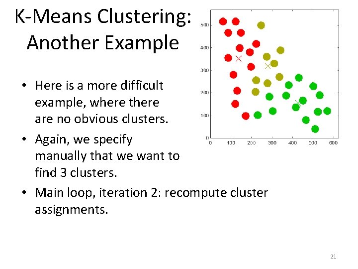
K-Means Clustering: Another Example • Here is a more difficult example, where there are no obvious clusters. • Again, we specify manually that we want to find 3 clusters. • Main loop, iteration 2: recompute cluster assignments. 21

K-Means Clustering: Another Example • Here is a more difficult example, where there are no obvious clusters. • Again, we specify manually that we want to find 3 clusters. • Main loop, iteration 3: recompute cluster assignments. 22

K-Means Clustering: Another Example • Here is a more difficult example, where there are no obvious clusters. • Again, we specify manually that we want to find 3 clusters. • Main loop, iteration 4: recompute cluster assignments. 23

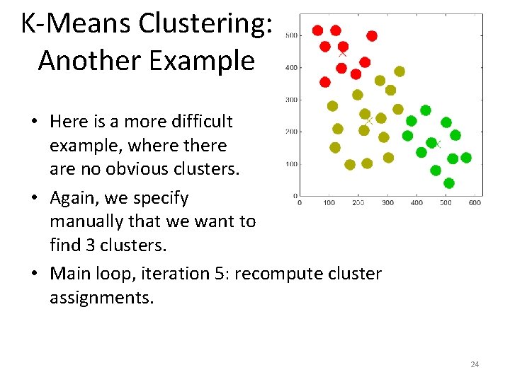
K-Means Clustering: Another Example • Here is a more difficult example, where there are no obvious clusters. • Again, we specify manually that we want to find 3 clusters. • Main loop, iteration 5: recompute cluster assignments. 24

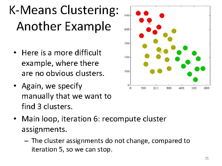
K-Means Clustering: Another Example • Here is a more difficult example, where there are no obvious clusters. • Again, we specify manually that we want to find 3 clusters. • Main loop, iteration 6: recompute cluster assignments. – The cluster assignments do not change, compared to iteration 5, so we can stop. 25

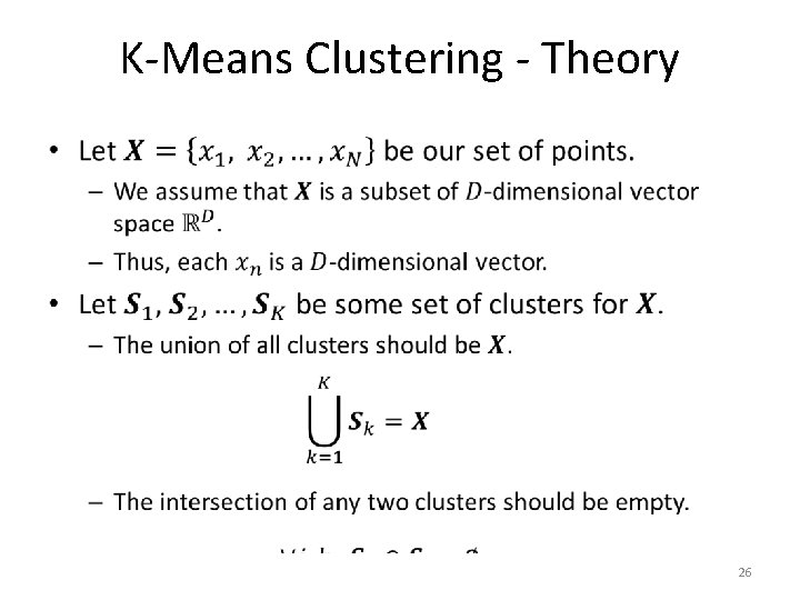
K-Means Clustering - Theory • 26

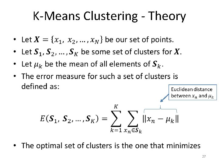
K-Means Clustering - Theory • 27

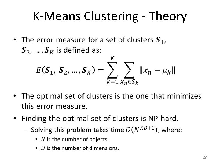
K-Means Clustering - Theory • 28

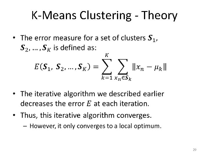
K-Means Clustering - Theory • 29

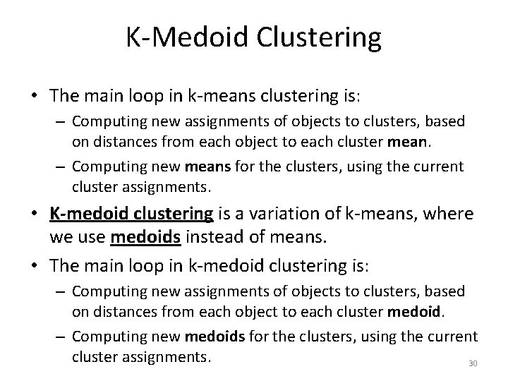
K-Medoid Clustering • The main loop in k-means clustering is: – Computing new assignments of objects to clusters, based on distances from each object to each cluster mean. – Computing new means for the clusters, using the current cluster assignments. • K-medoid clustering is a variation of k-means, where we use medoids instead of means. • The main loop in k-medoid clustering is: – Computing new assignments of objects to clusters, based on distances from each object to each cluster medoid. – Computing new medoids for the clusters, using the current cluster assignments. 30

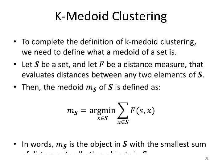
K-Medoid Clustering • 31

K-Medoid vs. K-means • K-medoid clustering can be applied on non-vector data with non-Euclidean distance measures. • For example: – K-medoid can be used to cluster a set of time series objects, using DTW as the distance measure. – K-medoid can be used to cluster a set of strings, using the edit distance as the distance measure. • K-means cannot be used in such cases. – Means may not make sense for non-vector data. – For example, it does not make sense to talk about the mean of a set of strings. However, we can define (and find) the medoid of a set of strings, under the edit distance. 32

K-Medoid vs. K-means • K-medoid clustering can be applied on non-vector data with non-Euclidean distance measures. • K-medoid clustering is more robust to outliers. – A single outlier can dominate the mean of a cluster, but it typically has only small influence on the medoid. • The K-means algorithm can be proven to converge to a local optimum. – The k-medoid algorithm may not converge. 33

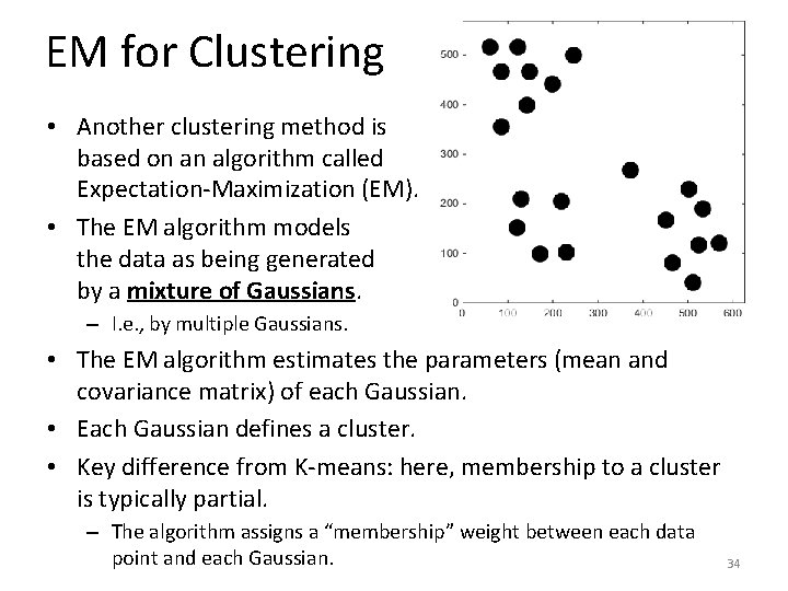
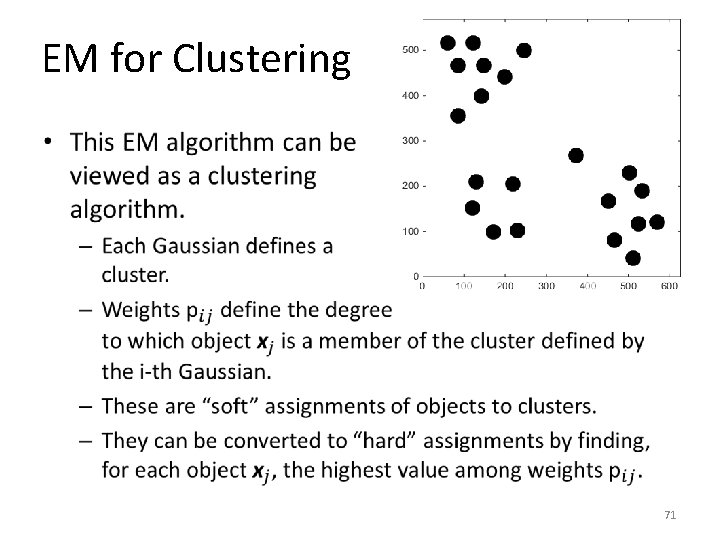
EM for Clustering • Another clustering method is based on an algorithm called Expectation-Maximization (EM). • The EM algorithm models the data as being generated by a mixture of Gaussians. – I. e. , by multiple Gaussians. • The EM algorithm estimates the parameters (mean and covariance matrix) of each Gaussian. • Each Gaussian defines a cluster. • Key difference from K-means: here, membership to a cluster is typically partial. – The algorithm assigns a “membership” weight between each data point and each Gaussian. 34

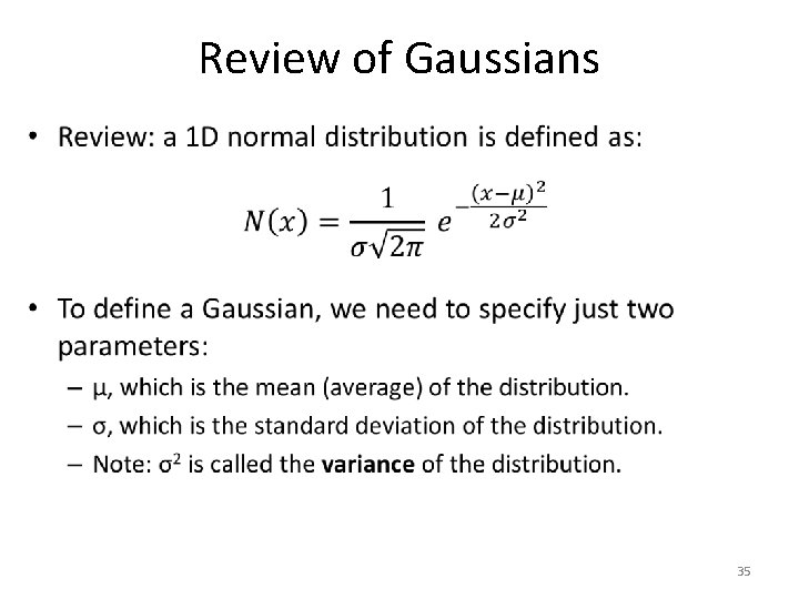
Review of Gaussians • 35

Estimating a Gaussian • 36

Estimating a Gaussian • Fitting a Gaussian to data does not guarantee that the resulting Gaussian will be an accurate distribution for the data. • The data may have a distribution that is very different from a Gaussian. 37

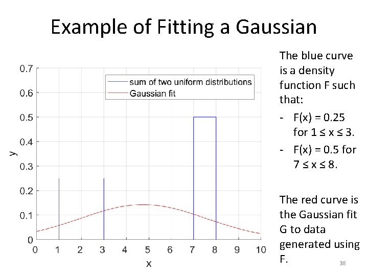
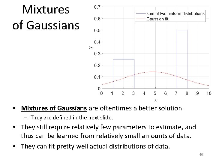
Example of Fitting a Gaussian The blue curve is a density function F such that: - F(x) = 0. 25 for 1 ≤ x ≤ 3. - F(x) = 0. 5 for 7 ≤ x ≤ 8. The red curve is the Gaussian fit G to data generated using F. 38

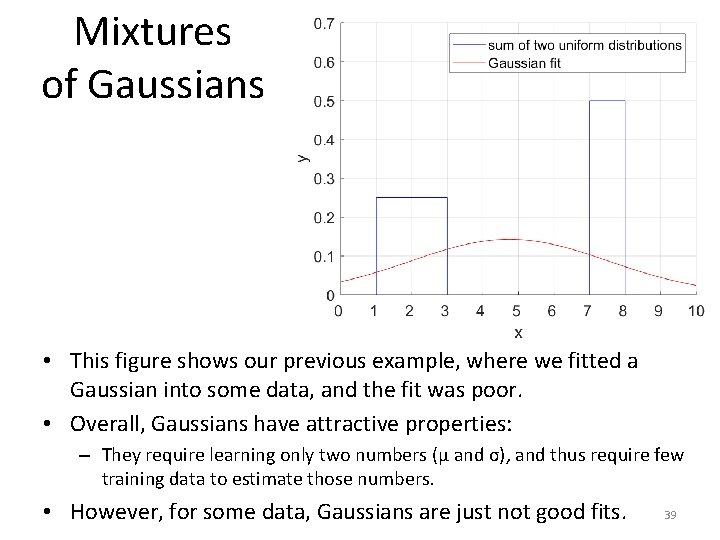
Mixtures of Gaussians • This figure shows our previous example, where we fitted a Gaussian into some data, and the fit was poor. • Overall, Gaussians have attractive properties: – They require learning only two numbers (μ and σ), and thus require few training data to estimate those numbers. • However, for some data, Gaussians are just not good fits. 39

Mixtures of Gaussians • Mixtures of Gaussians are oftentimes a better solution. – They are defined in the next slide. • They still require relatively few parameters to estimate, and thus can be learned from relatively small amounts of data. • They can fit pretty well actual distributions of data. 40

Mixtures of Gaussians • 41

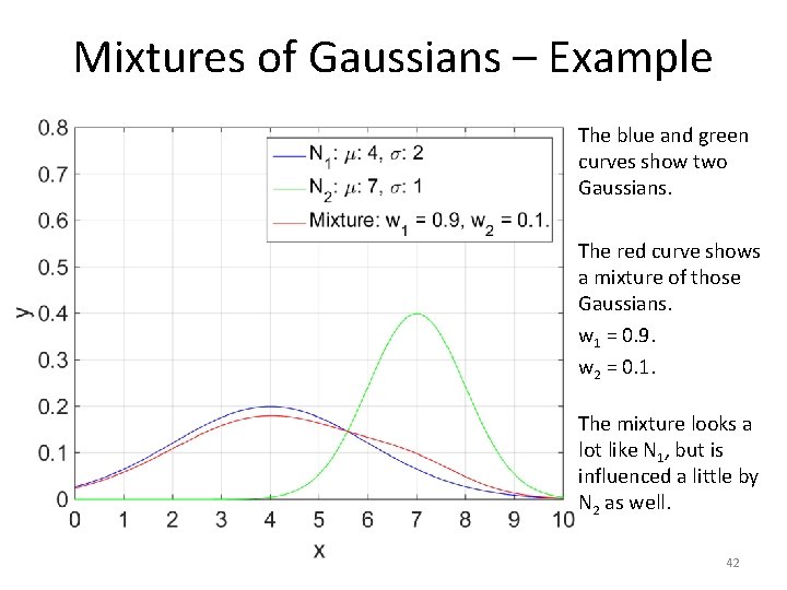
Mixtures of Gaussians – Example The blue and green curves show two Gaussians. The red curve shows a mixture of those Gaussians. w 1 = 0. 9. w 2 = 0. 1. The mixture looks a lot like N 1, but is influenced a little by N 2 as well. 42

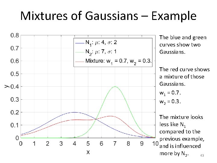
Mixtures of Gaussians – Example The blue and green curves show two Gaussians. The red curve shows a mixture of those Gaussians. w 1 = 0. 7. w 2 = 0. 3. The mixture looks less like N 1 compared to the previous example, and is influenced more by N 2. 43

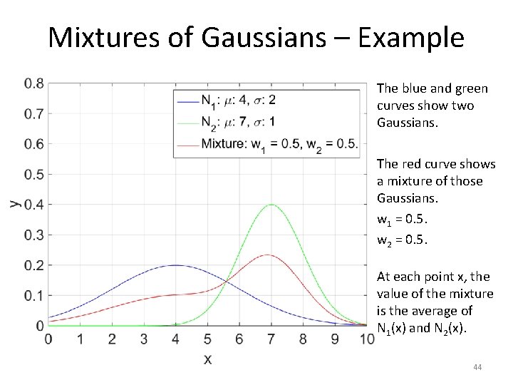
Mixtures of Gaussians – Example The blue and green curves show two Gaussians. The red curve shows a mixture of those Gaussians. w 1 = 0. 5. w 2 = 0. 5. At each point x, the value of the mixture is the average of N 1(x) and N 2(x). 44

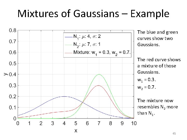
Mixtures of Gaussians – Example The blue and green curves show two Gaussians. The red curve shows a mixture of those Gaussians. w 1 = 0. 3. w 2 = 0. 7. The mixture now resembles N 2 more than N 1. 45

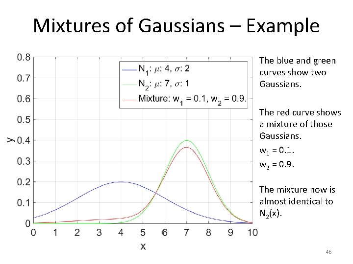
Mixtures of Gaussians – Example The blue and green curves show two Gaussians. The red curve shows a mixture of those Gaussians. w 1 = 0. 1. w 2 = 0. 9. The mixture now is almost identical to N 2(x). 46

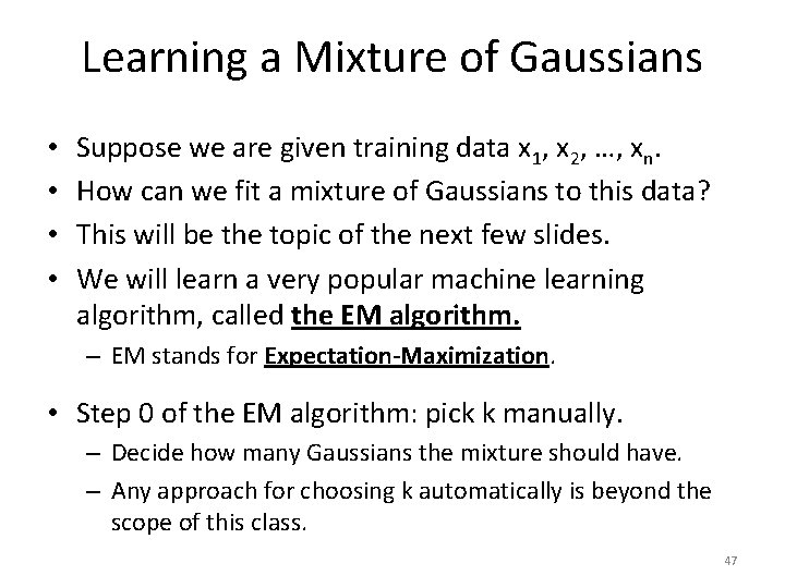
Learning a Mixture of Gaussians • • Suppose we are given training data x 1, x 2, …, xn. How can we fit a mixture of Gaussians to this data? This will be the topic of the next few slides. We will learn a very popular machine learning algorithm, called the EM algorithm. – EM stands for Expectation-Maximization. • Step 0 of the EM algorithm: pick k manually. – Decide how many Gaussians the mixture should have. – Any approach for choosing k automatically is beyond the scope of this class. 47

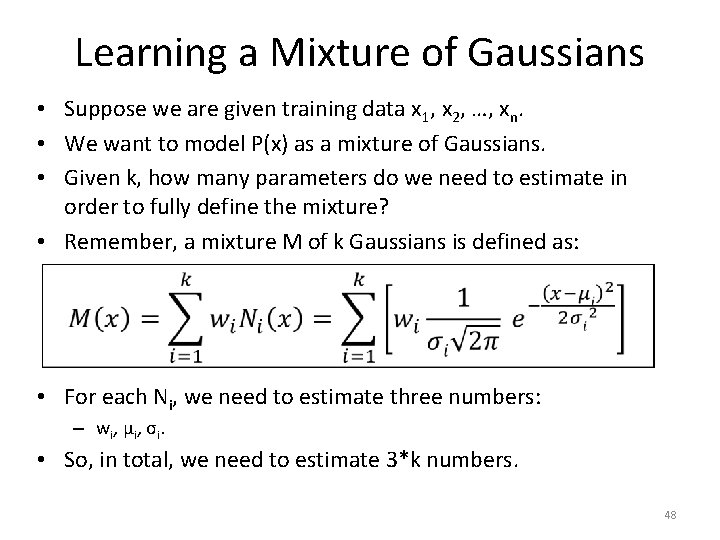
Learning a Mixture of Gaussians • Suppose we are given training data x 1, x 2, …, xn. • We want to model P(x) as a mixture of Gaussians. • Given k, how many parameters do we need to estimate in order to fully define the mixture? • Remember, a mixture M of k Gaussians is defined as: • For each Ni, we need to estimate three numbers: – wi, μi, σi. • So, in total, we need to estimate 3*k numbers. 48

Learning a Mixture of Gaussians • Suppose we are given training data x 1, x 2, …, xn. • A mixture M of k Gaussians is defined as: • For each Ni, we need to estimate wi, μi, σi. • Suppose that we knew for each xj, that it belongs to one and only one of the k Gaussians. • Then, learning the mixture would be a piece of cake: • For each Gaussian Ni: – Estimate μi, σi based on the examples that belong to it. – Set wi equal to the fraction of examples that belong to Ni. 49

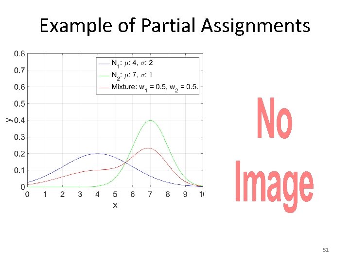
Learning a Mixture of Gaussians • Suppose we are given training data x 1, x 2, …, xn. • A mixture M of k Gaussians is defined as: • For each Ni, we need to estimate wi, μi, σi. • However, we have no idea which mixture each xj belongs to. • If we knew μi and σi for each Ni, we could probabilistically assign each xj to a component. – “Probabilistically” means that we would not make a hard assignment, but we would partially assign xj to different components, with each assignment weighted proportionally to the density value Ni(xj). 50

Example of Partial Assignments • 51

The Chicken-and-Egg Problem • To recap, fitting a mixture of Gaussians to data involves estimating, for each Ni, values wi, μi, σi. • If we could assign each xj to one of the Gaussians, we could compute easily wi, μi, σi. – Even if we probabilistically assign xj to multiple Gaussians, we can still easily wi, μi, σi, by adapting our previous formulas. We will see the adapted formulas in a few slides. • If we knew μi, σi and wi, we could assign (at least probabilistically) xj’s to Gaussians. • So, this is a chicken-and-egg problem. – If we knew one piece, we could compute the other. – But, we know neither. So, what do we do? 52

On Chicken-and-Egg Problems • Such chicken-and-egg problems occur frequently in AI. • Surprisingly (at least to people new in AI), we can easily solve such chicken-and-egg problems. • Overall, chicken and egg problems in AI look like this: – We need to know A to estimate B. – We need to know B to compute A. • There is a fairly standard recipe for solving these problems. • Any guesses? 53

On Chicken-and-Egg Problems • Such chicken-and-egg problems occur frequently in AI. • Surprisingly (at least to people new in AI), we can easily solve such chicken-and-egg problems. • Overall, chicken and egg problems in AI look like this: – We need to know A to estimate B. – We need to know B to compute A. • There is a fairly standard recipe for solving these problems. • Start by giving to A values chosen randomly (or perhaps nonrandomly, but still in an uninformed way, since we do not know the correct values). • Repeat this loop: – Given our current values for A, estimate B. – Given our current values of B, estimate A. – If the new values of A and B are very close to the old values, break. 54

The EM Algorithm - Overview • We use this approach to fit mixtures of Gaussians to data. • This algorithm, that fits mixtures of Gaussians to data, is called the EM algorithm (Expectation-Maximization algorithm). • Remember, we choose k (the number of Gaussians in the mixture) manually, so we don’t have to estimate that. • To initialize the EM algorithm, we initialize each μi, σi, and wi. Values wi are set to 1/k. We can initialize μi, σi in different ways: – – Giving random values to each μi. Uniformly spacing the values given to each μi. Giving random values to each σi. Setting each σi to 1 initially. • Then, we iteratively perform two steps. – The E-step. – The M-step. 55

The E-Step • 56

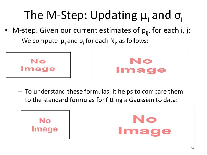
The M-Step: Updating μi and σi • M-step. Given our current estimates of pij, for each i, j: – We compute μi and σi for each Ni, as follows: – To understand these formulas, it helps to compare them to the standard formulas for fitting a Gaussian to data: 57

The M-Step: Updating μi and σi – To understand these formulas, it helps to compare them to the standard formulas for fitting a Gaussian to data: • 58

The M-Step: Updating wi • 59

The EM Steps: Summary • 60

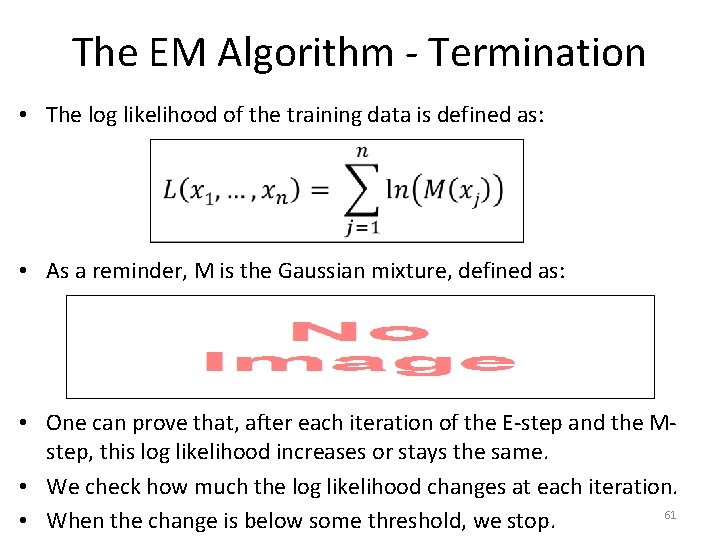
The EM Algorithm - Termination • The log likelihood of the training data is defined as: • As a reminder, M is the Gaussian mixture, defined as: • One can prove that, after each iteration of the E-step and the Mstep, this log likelihood increases or stays the same. • We check how much the log likelihood changes at each iteration. 61 • When the change is below some threshold, we stop.

The EM Algorithm: Summary • 62

The EM Algorithm: Limitations • When we fit a Gaussian to data, we always get the same result. • We can also prove that the result that we get is the best possible result. – There is no other Gaussian giving a higher log likelihood to the data, than the one that we compute as described in these slides. • When we fit a mixture of Gaussians to the same data, do we always end up with the same result? 63

The EM Algorithm: Limitations • When we fit a Gaussian to data, we always get the same result. • We can also prove that the result that we get is the best possible result. – There is no other Gaussian giving a higher log likelihood to the data, than the one that we compute as described in these slides. • When we fit a mixture of Gaussians to the same data, we (sadly) do not always get the same result. • The EM algorithm is a greedy algorithm. • The result depends on the initialization values. • We may have bad luck with the initial values, and end up with a bad fit. • There is no good way to know if our result is good or bad, or if better results are possible. 64

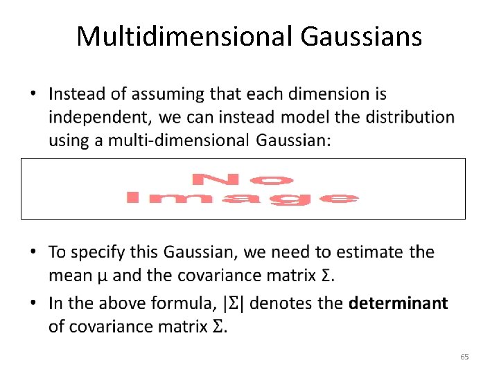
Multidimensional Gaussians • 65

Multidimensional Gaussians - Mean • 66

Multidimensional Gaussians – Covariance Matrix • • Let x 1, x 2, …, xn be d-dimensional vectors. xi = (xi, 1, xi, 2, …, xi, d), where each xi, j is a real number. Let Σ be the covariance matrix. Its size is dxd. Let σr, c be the value of Σ at row r, column c. 67

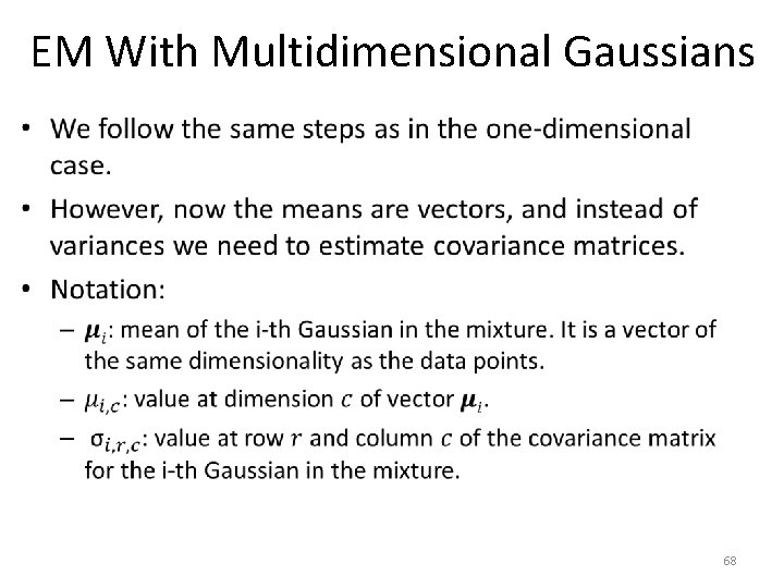
EM With Multidimensional Gaussians • 68

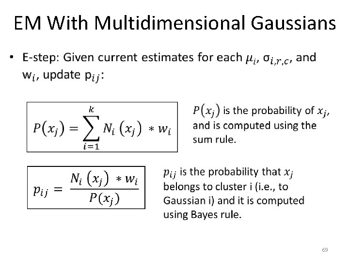
EM With Multidimensional Gaussians • 69

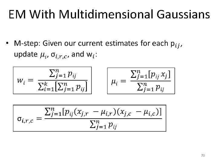
EM With Multidimensional Gaussians • 70

EM for Clustering • 71

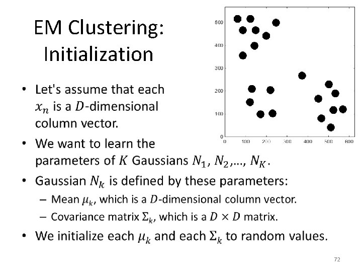
EM Clustering: Initialization • 72

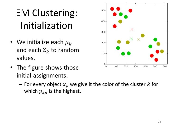
EM Clustering: Initialization • 73

EM Clustering: Main Loop • 74

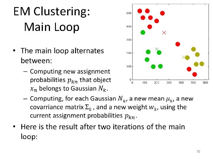
EM Clustering: Main Loop • 75

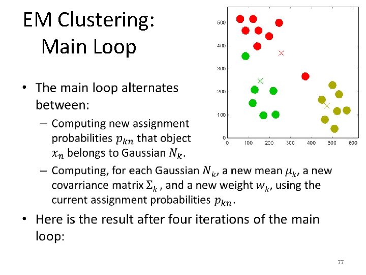
EM Clustering: Main Loop • 76

EM Clustering: Main Loop • 77

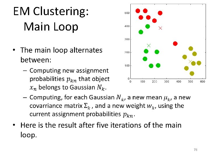
EM Clustering: Main Loop • 78

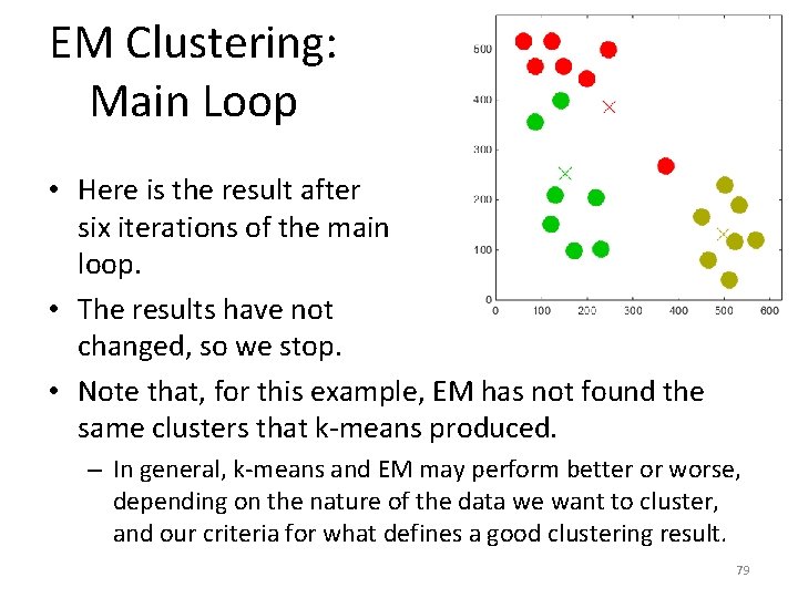
EM Clustering: Main Loop • Here is the result after six iterations of the main loop. • The results have not changed, so we stop. • Note that, for this example, EM has not found the same clusters that k-means produced. – In general, k-means and EM may perform better or worse, depending on the nature of the data we want to cluster, and our criteria for what defines a good clustering result. 79

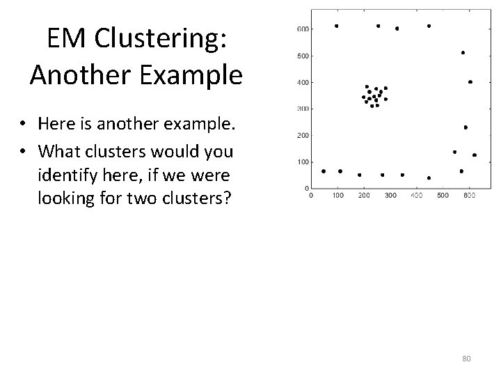
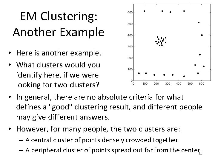
EM Clustering: Another Example • Here is another example. • What clusters would you identify here, if we were looking for two clusters? 80

EM Clustering: Another Example • Here is another example. • What clusters would you identify here, if we were looking for two clusters? • In general, there are no absolute criteria for what defines a "good" clustering result, and different people may give different answers. • However, for many people, the two clusters are: – A central cluster of points densely crowded together. – A peripheral cluster of points spread out far from the center. 81

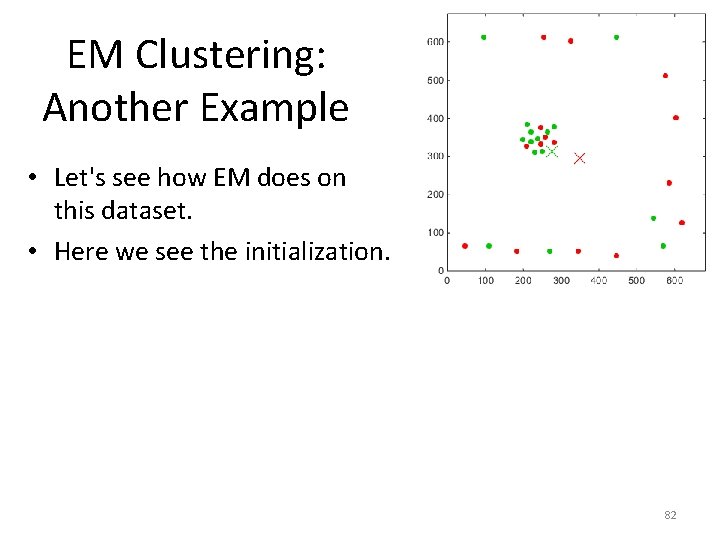
EM Clustering: Another Example • Let's see how EM does on this dataset. • Here we see the initialization. 82

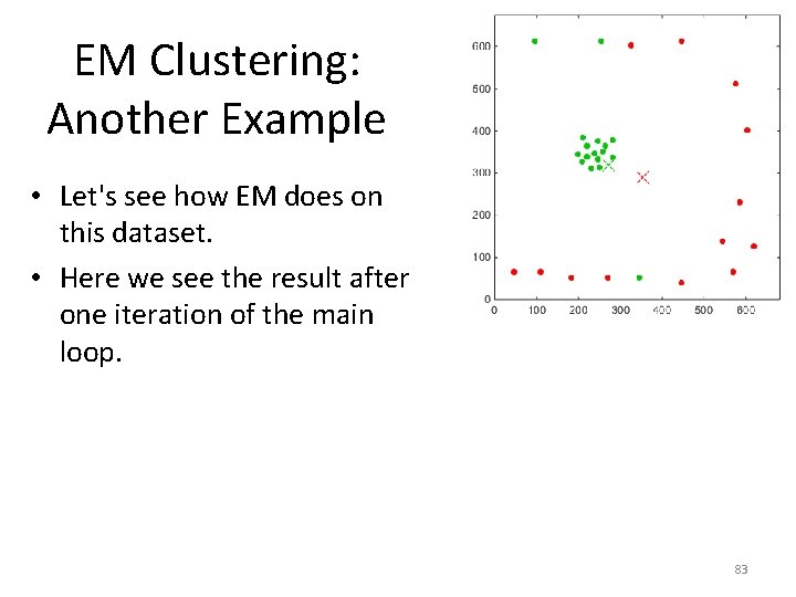
EM Clustering: Another Example • Let's see how EM does on this dataset. • Here we see the result after one iteration of the main loop. 83

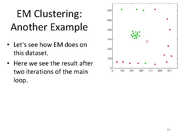
EM Clustering: Another Example • Let's see how EM does on this dataset. • Here we see the result after two iterations of the main loop. 84

EM Clustering: Another Example • Let's see how EM does on this dataset. • Here we see the result after three iterations of the main loop. 85

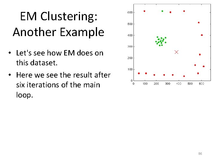
EM Clustering: Another Example • Let's see how EM does on this dataset. • Here we see the result after six iterations of the main loop. 86

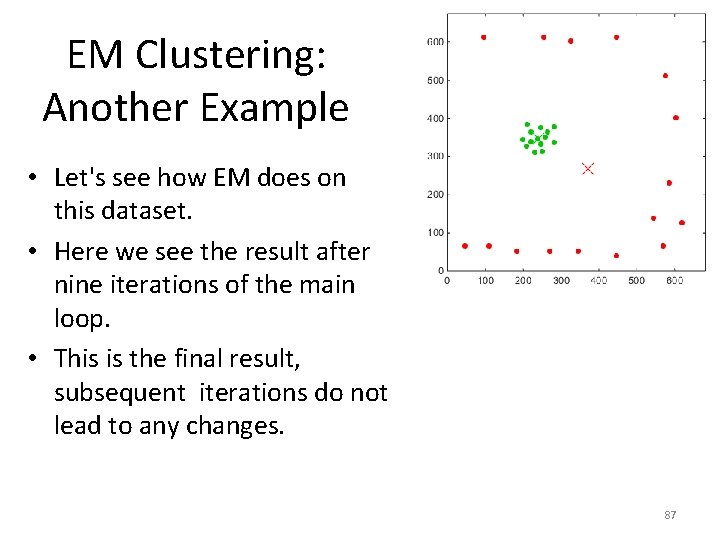
EM Clustering: Another Example • Let's see how EM does on this dataset. • Here we see the result after nine iterations of the main loop. • This is the final result, subsequent iterations do not lead to any changes. 87

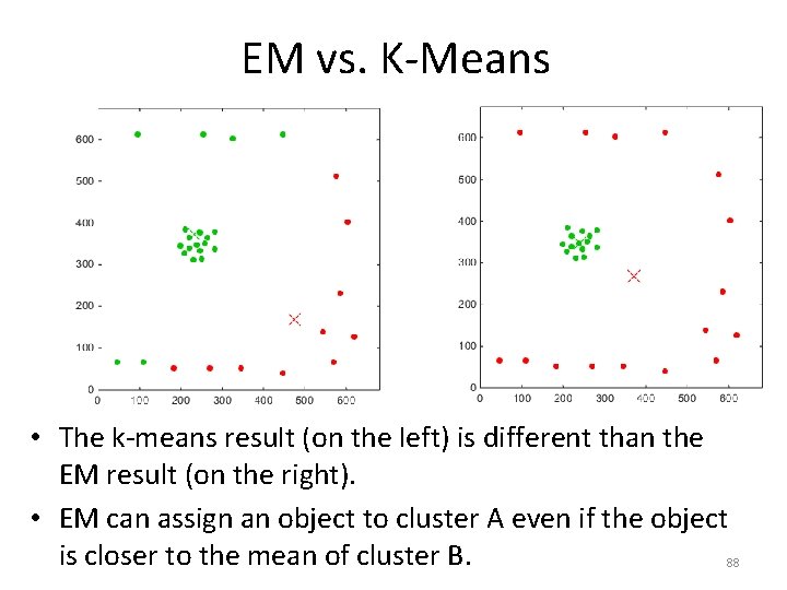
EM vs. K-Means • The k-means result (on the left) is different than the EM result (on the right). • EM can assign an object to cluster A even if the object is closer to the mean of cluster B. 88

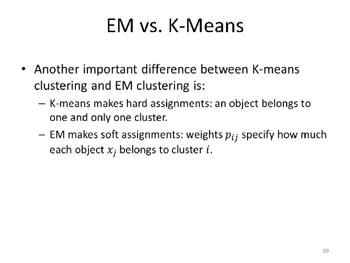
EM vs. K-Means • 89

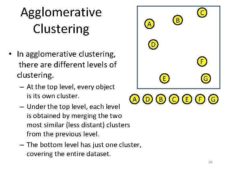
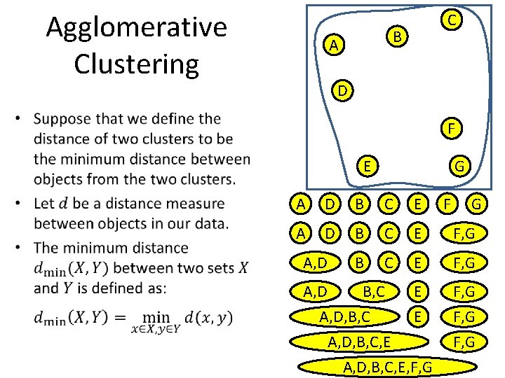
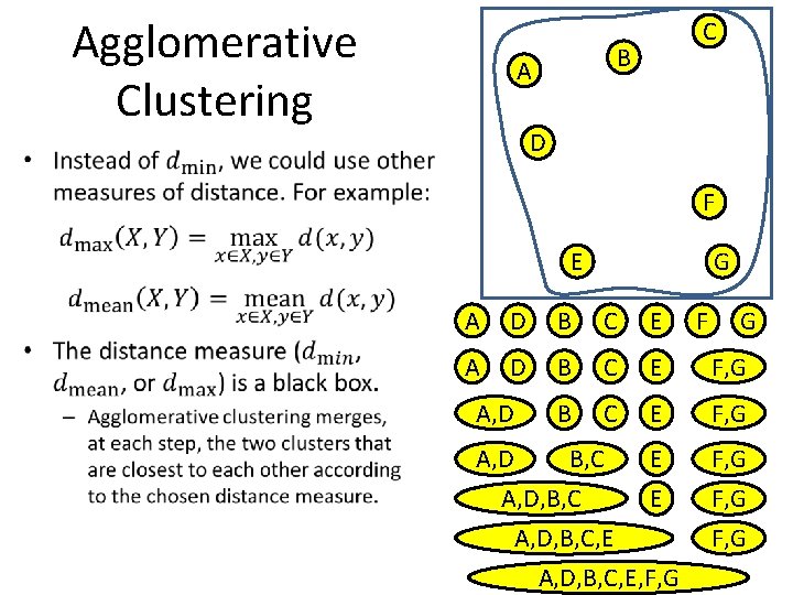
Agglomerative Clustering B A • In agglomerative clustering, there are different levels of clustering. – At the top level, every object is its own cluster. A D – Under the top level, each level is obtained by merging the two most similar (less distant) clusters from the previous level. – The bottom level has just one cluster, covering the entire dataset. C D F E B G C E F G 90

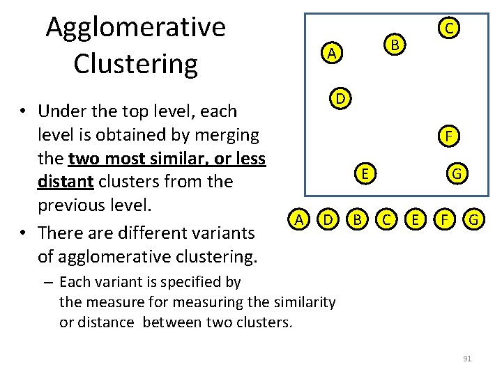
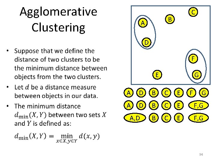
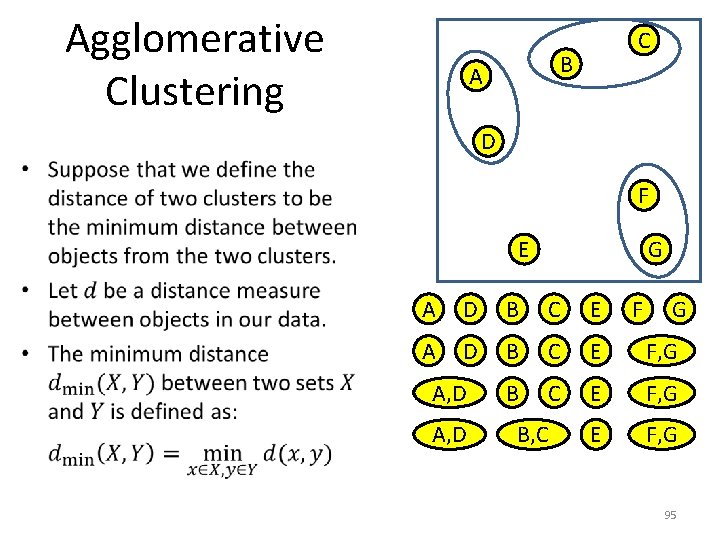
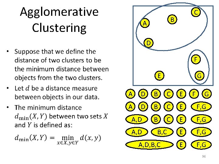
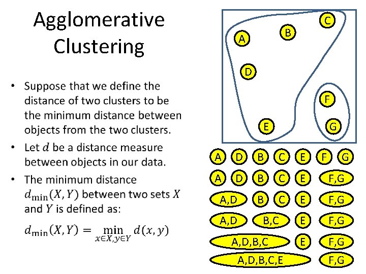
Agglomerative Clustering • Under the top level, each level is obtained by merging the two most similar, or less distant clusters from the previous level. • There are different variants of agglomerative clustering. C B A D F E A D B G C E F G – Each variant is specified by the measure for measuring the similarity or distance between two clusters. 91

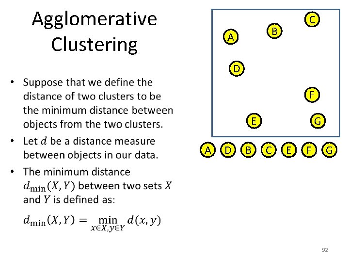
Agglomerative Clustering C B A D • F E A D B G C E F G 92

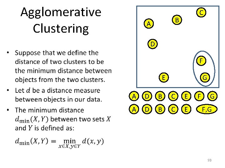
Agglomerative Clustering C B A D • F E G A D B C E F G F, G 93

Agglomerative Clustering C B A D • F E G A D B C E F, G A, D F G 94

Agglomerative Clustering C B A D • F E G A D B C E F, G A, D B, C F G 95

Agglomerative Clustering C B A D • F E G A D B C E F, G E F, G A, D B, C A, D, B, C F G 96

Agglomerative Clustering C B A D • F E G A D B C E F, G E F, G 97 F, G A, D B, C A, D, B, C, E F G

Agglomerative Clustering C B A D • F E G A D B C E F, G A, D B, C E A, D, B, C, E, F, G F, G 98

Agglomerative Clustering C B A D • F E G A D B C E F, G A, D B, C E A, D, B, C, E, F, G F, G 99

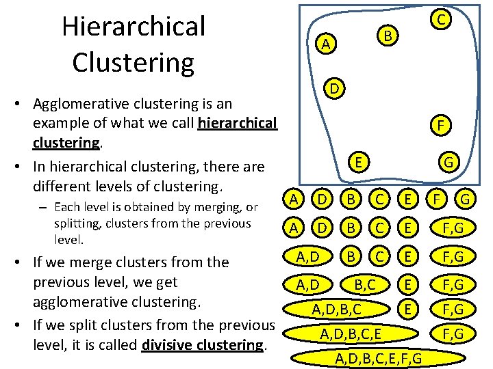
Hierarchical Clustering • Agglomerative clustering is an example of what we call hierarchical clustering. • In hierarchical clustering, there are different levels of clustering. – Each level is obtained by merging, or splitting, clusters from the previous level. C B A D F E G A D B C E A, D B C E • If we merge clusters from the previous level, we get A, D B, C E agglomerative clustering. A, D, B, C E • If we split clusters from the previous A, D, B, C, E level, it is called divisive clustering. A, D, B, C, E, F, G F, G 100

Clustering - Recap • The goal in clustering is to split a set of objects into groups of similar objects. • There is no single criterion for measuring the quality of a clustering result. • The number of clusters typically needs to be specified in advance. – Methods (that we have not seen) do exist for trying to find the number of clusters automatically. – In hierarchical clustering (e. g. , agglomerative clustering), we do not need to pick a number of clusters. • A large variety of clustering methods exist. • We saw a few examples of such methods: – K-means, K-medoid, EM, agglomerative clustering. 101