Clustering Hierarchical Agglomerative and Point Assignment Approaches Measures

Clustering Hierarchical /Agglomerative and Point. Assignment Approaches Measures of “Goodness” for Clusters BFR Algorithm CURE Algorithm Jeffrey D. Ullman Stanford University

The Problem of Clustering �Given a set of points, with a notion of distance between points, group the points into some number of clusters, so that members of a cluster are “close” to each other, while members of different clusters are “far. ” 2

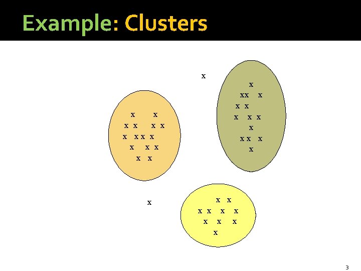
Example: Clusters x x x x xx x x x x x x 3

Problems With Clustering �Clustering in two dimensions looks easy. �Clustering small amounts of data looks easy. �And in most cases, looks are not deceiving. 4

The Curse of Dimensionality �Many applications involve not 2, but 10 or 10, 000 dimensions. �High-dimensional spaces look different: almost all pairs of points are at about the same distance. 5

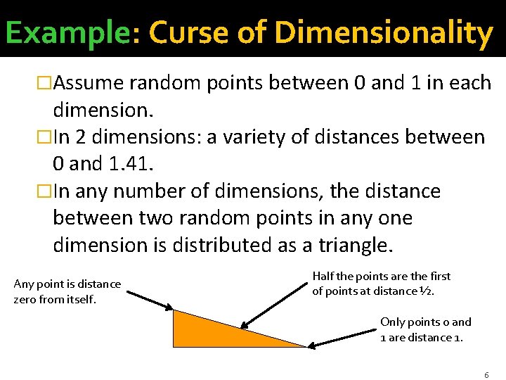
Example: Curse of Dimensionality �Assume random points between 0 and 1 in each dimension. �In 2 dimensions: a variety of distances between 0 and 1. 41. �In any number of dimensions, the distance between two random points in any one dimension is distributed as a triangle. Any point is distance zero from itself. Half the points are the first of points at distance ½. Only points 0 and 1 are distance 1. 6

Example – Continued �The law of large numbers applies. �Actual distance between two random points is the sqrt of the sum of squares of essentially the same set of differences. § I. e. , “all points are the same distance apart. ” 7

Euclidean and Non-Euclidean Distances �Euclidean spaces have dimensions, and points have coordinates in each dimension. �Distance between points is usually the squareroot of the sum of the squares of the distances in each dimension. �Non-Euclidean spaces have a distance measure, but points do not really have a position in the space. § Big problem: cannot “average” points. 8

Example: DNA Sequences �Objects are sequences of {C, A, T, G}. �Distance between sequences = edit distance = the minimum number of inserts and deletes needed to turn one into the other. § Notice: no way to “average” two strings. �In practice, the distance for DNA sequences is more complicated: allows other operations like mutations (change of a symbol into another) or reversal of substrings. 9

Methods of Clustering �Hierarchical (Agglomerative): § Initially, each point in cluster by itself. § Repeatedly combine the two “nearest” clusters into one. �Point Assignment: § Maintain a set of clusters. § Place points into their “nearest” cluster. § Possibly split clusters or combine clusters as we go. 10

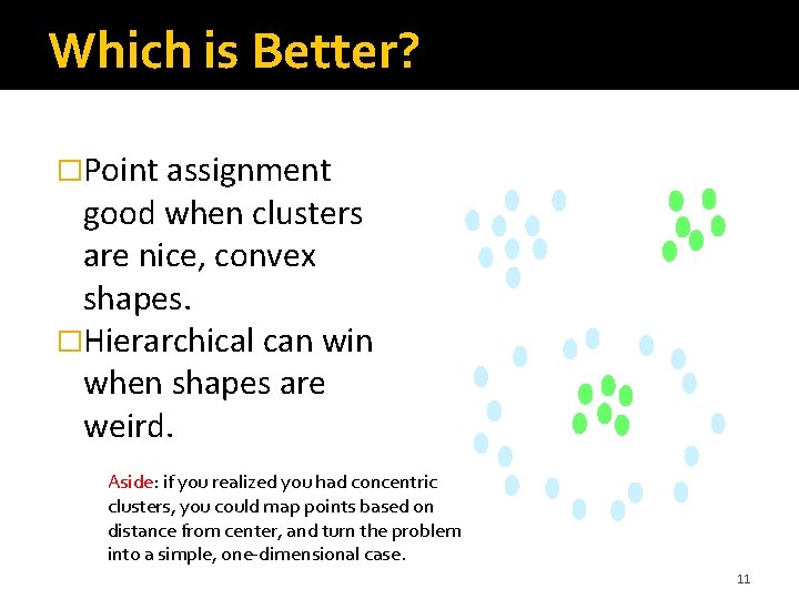
Which is Better? �Point assignment good when clusters are nice, convex shapes. �Hierarchical can win when shapes are weird. Aside: if you realized you had concentric clusters, you could map points based on distance from center, and turn the problem into a simple, one-dimensional case. 11

Hierarchical Clustering � Two important questions: 1. How do you determine the “nearness” of clusters? 2. How do you represent a cluster of more than one point? 12

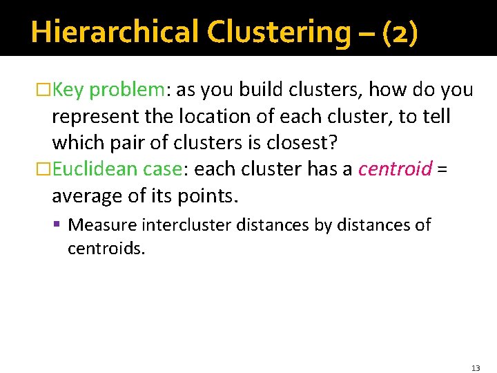
Hierarchical Clustering – (2) �Key problem: as you build clusters, how do you represent the location of each cluster, to tell which pair of clusters is closest? �Euclidean case: each cluster has a centroid = average of its points. § Measure intercluster distances by distances of centroids. 13

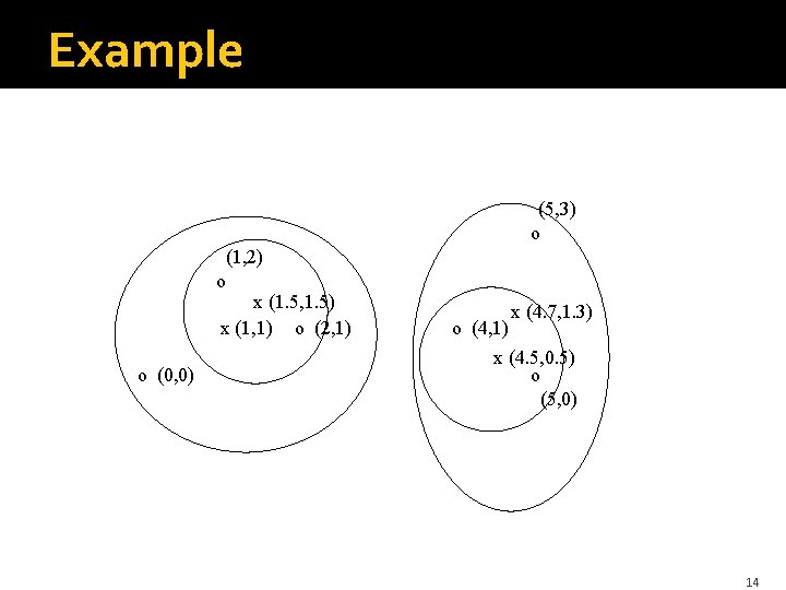
Example (5, 3) o (1, 2) o x (1. 5, 1. 5) x (1, 1) o (2, 1) o (0, 0) o (4, 1) x (4. 7, 1. 3) x (4. 5, 0. 5) o (5, 0) 14

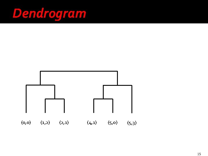
Dendrogram (0, 0) (1, 2) (2, 1) (4, 1) (5, 0) (5, 3) 15

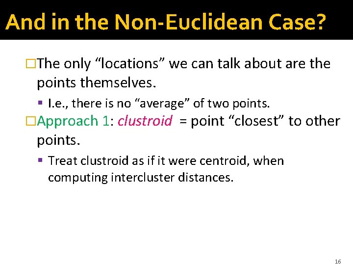
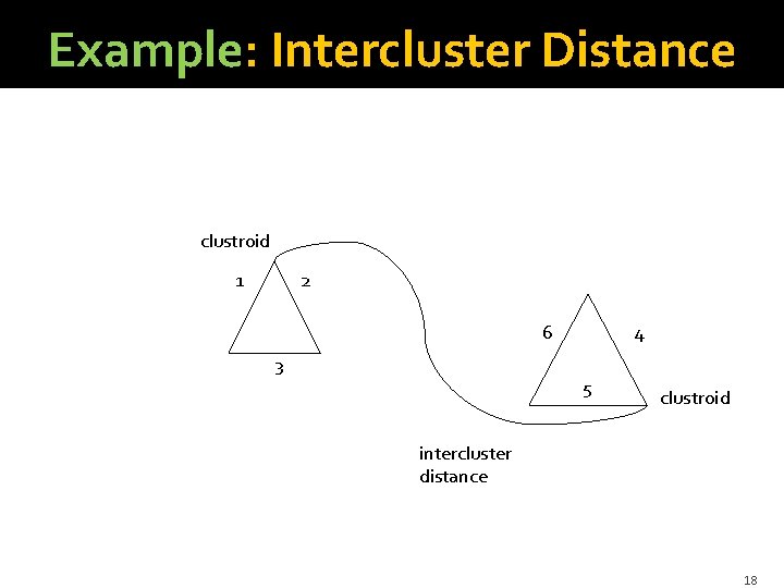
And in the Non-Euclidean Case? �The only “locations” we can talk about are the points themselves. § I. e. , there is no “average” of two points. �Approach 1: clustroid points. = point “closest” to other § Treat clustroid as if it were centroid, when computing intercluster distances. 16

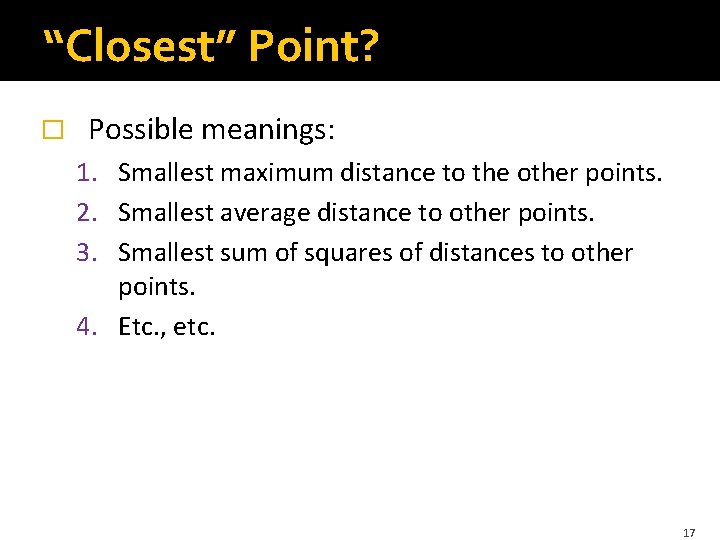
“Closest” Point? � Possible meanings: 1. Smallest maximum distance to the other points. 2. Smallest average distance to other points. 3. Smallest sum of squares of distances to other points. 4. Etc. , etc. 17

Example: Intercluster Distance clustroid 1 2 6 3 4 5 clustroid intercluster distance 18

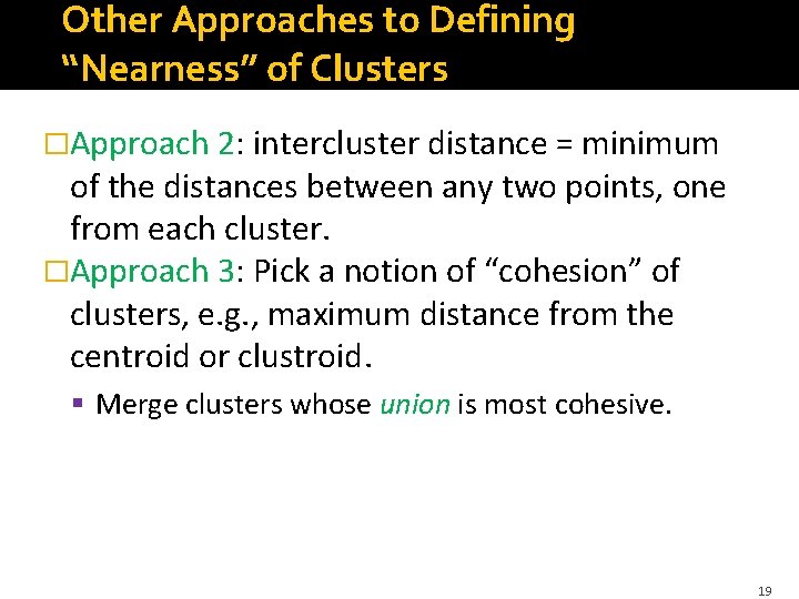
Other Approaches to Defining “Nearness” of Clusters �Approach 2: intercluster distance = minimum of the distances between any two points, one from each cluster. �Approach 3: Pick a notion of “cohesion” of clusters, e. g. , maximum distance from the centroid or clustroid. § Merge clusters whose union is most cohesive. 19

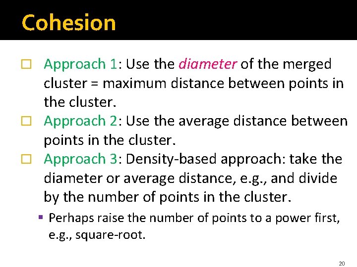
Cohesion Approach 1: Use the diameter of the merged cluster = maximum distance between points in the cluster. � Approach 2: Use the average distance between points in the cluster. � Approach 3: Density-based approach: take the diameter or average distance, e. g. , and divide by the number of points in the cluster. � § Perhaps raise the number of points to a power first, e. g. , square-root. 20

Which is Best �It really depends on the shape of clusters. § Which you may not know in advance. �Example: we’ll compare two approaches: 1. Merge clusters with smallest distance between centroids (or clustroids for non-Euclidean). 2. Merge clusters with the smallest distance between two points, one from each cluster. 21

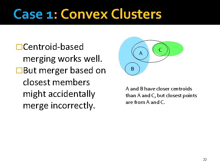
Case 1: Convex Clusters �Centroid-based merging works well. �But merger based on closest members might accidentally merge incorrectly. A C B A and B have closer centroids than A and C, but closest points are from A and C. 22

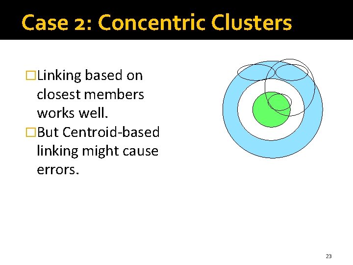
Case 2: Concentric Clusters �Linking based on closest members works well. �But Centroid-based linking might cause errors. 23

k–Means Algorithm(s) �An example of point-assignment. �Assumes Euclidean space. �Start by picking k, the number of clusters. �Initialize clusters with a seed (= one point per cluster). § Example: pick one point at random, then k-1 other points, each as far away as possible from the previous points. § OK, as long as there are no outliers (points that are far from any reasonable cluster). 24

k-Means++ �Basic idea: pick a small sample of points, cluster them by any algorithm, and use the centroids as a seed. �In k-means++, sample size = k times a factor that is logarithmic in the total number of points. �Sequentially pick sample points randomly, but the probability of adding a point p to the sample is proportional to D(p)2. § D(p) = distance between p and the nearest picked point. 25

k-Means | | �k-means++, like other seed methods, is sequential. § You need to update D(p) for each unpicked p due to new point. �Naturally parallel: many compute nodes can each handle a small set of points. § Each picks a few new sample points using same D(p). �Really important and common trick: don’t update after every selection; rather make many selections at one round. § Suboptimal picks don’t really matter. 26

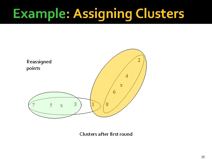
Populating Clusters For each point, place it in the cluster whose current centroid it is nearest. 2. After all points are assigned, fix the centroids of the k clusters. 3. Optional: reassign all points to their closest centroid. 1. § Sometimes moves points between clusters. 27

Example: Assigning Clusters 2 Reassigned points 4 x 6 7 5 x 3 1 8 Clusters after first round 28

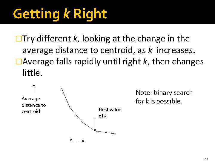
Getting k Right �Try different k, looking at the change in the average distance to centroid, as k increases. �Average falls rapidly until right k, then changes little. Note: binary search for k is possible. Average distance to centroid Best value of k k 29

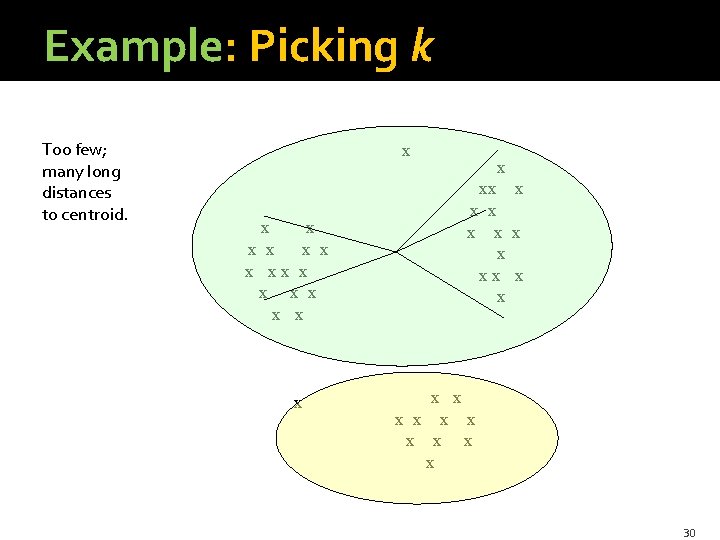
Example: Picking k Too few; many long distances to centroid. x x x x xx x x x x x x 30

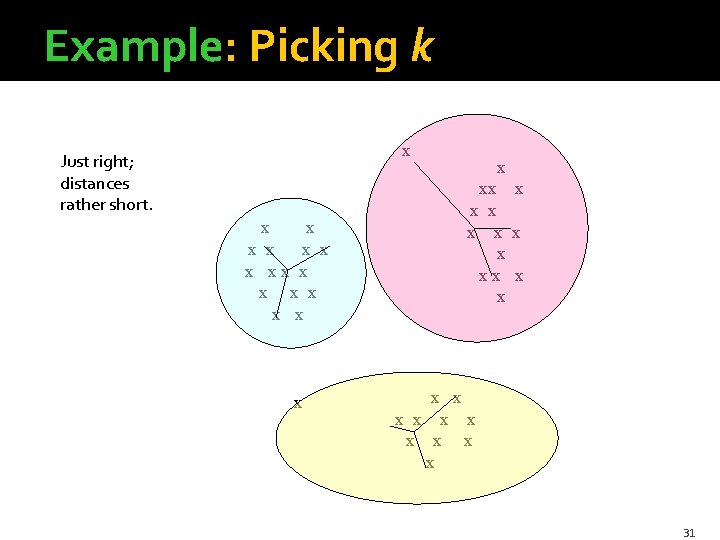
Example: Picking k x Just right; distances rather short. x x x xx x xx x x x 31

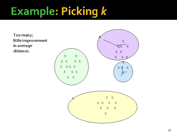
Example: Picking k Too many; little improvement in average distance. x x x x xx x x x x x x 32

BFR Algorithm �BFR (Bradley-Fayyad-Reina) is a variant of k- means designed to handle very large (diskresident) data sets. �It assumes that clusters are normally distributed around a centroid in a Euclidean space. § Standard deviations in different dimensions may vary. 33

BFR – (2) �Points are read one main-memory-full at a time. �Most points from previous memory loads are summarized by simple statistics. § Also kept in main memory, which limits how many points can be read in one “memory load. ” �To begin, from the initial load we select the initial k centroids by some sensible approach. 34

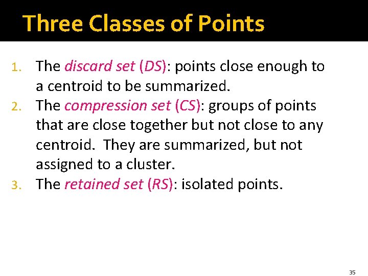
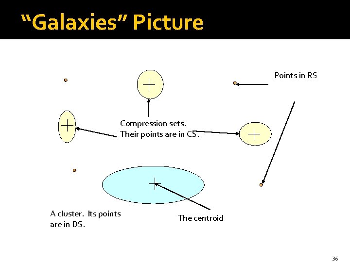
Three Classes of Points The discard set (DS): points close enough to a centroid to be summarized. 2. The compression set (CS): groups of points that are close together but not close to any centroid. They are summarized, but not assigned to a cluster. 3. The retained set (RS): isolated points. 1. 35

“Galaxies” Picture Points in RS Compression sets. Their points are in CS. A cluster. Its points are in DS. The centroid 36

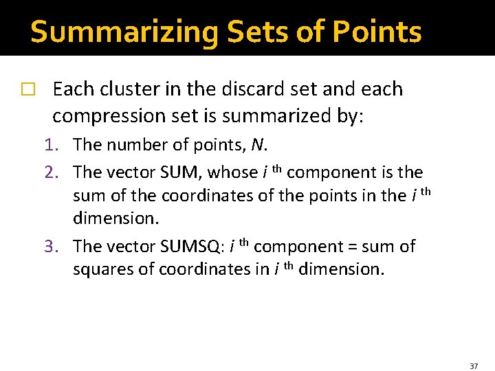
Summarizing Sets of Points � Each cluster in the discard set and each compression set is summarized by: 1. The number of points, N. 2. The vector SUM, whose i th component is the sum of the coordinates of the points in the i th dimension. 3. The vector SUMSQ: i th component = sum of squares of coordinates in i th dimension. 37

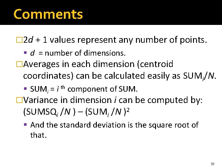
Comments � 2 d + 1 values represent any number of points. § d = number of dimensions. �Averages in each dimension (centroid coordinates) can be calculated easily as SUMi/N. § SUMi = i th component of SUM. �Variance in dimension i can be computed by: (SUMSQi /N ) – (SUMi /N )2 § And the standard deviation is the square root of that. 38

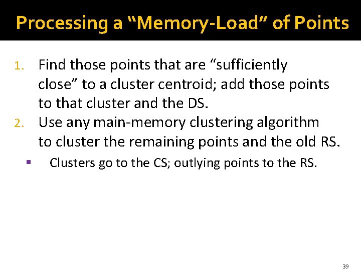
Processing a “Memory-Load” of Points Find those points that are “sufficiently close” to a cluster centroid; add those points to that cluster and the DS. 2. Use any main-memory clustering algorithm to cluster the remaining points and the old RS. 1. § Clusters go to the CS; outlying points to the RS. 39

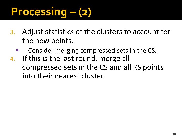
Processing – (2) Adjust statistics of the clusters to account for the new points. 3. § 4. Consider merging compressed sets in the CS. If this is the last round, merge all compressed sets in the CS and all RS points into their nearest cluster. 40

A Few Details. . . �How do we decide if a point is “close enough” to a cluster that we will add the point to that cluster? �How do we decide whether two compressed sets deserve to be combined into one? 41

How Close is Close Enough? We need a way to decide whether to put a new point into a cluster. � BFR suggest two ways: � 1. The Mahalanobis distance is less than a threshold. 2. Low likelihood of the currently nearest centroid changing. 42

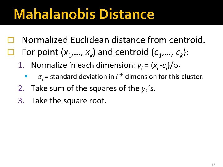
Mahalanobis Distance � � Normalized Euclidean distance from centroid. For point (x 1, …, xk) and centroid (c 1, …, ck): 1. Normalize in each dimension: yi = (xi -ci)/ i § i = standard deviation in i th dimension for this cluster. 2. Take sum of the squares of the yi ’s. 3. Take the square root. 43

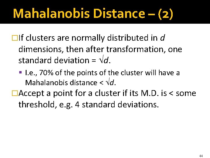
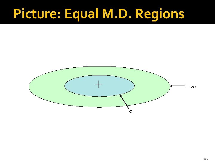
Mahalanobis Distance – (2) �If clusters are normally distributed in d dimensions, then after transformation, one standard deviation = d. § I. e. , 70% of the points of the cluster will have a Mahalanobis distance < d. �Accept a point for a cluster if its M. D. is < some threshold, e. g. 4 standard deviations. 44

Picture: Equal M. D. Regions 2 45

Should Two CS Subclusters Be Combined? �Similar to measuring cohesion. For example: �Compute the variance of the combined subcluster, in each dimension. § N, SUM, and SUMSQ allow us to make that calculation quickly. �Combine if the variance is below some threshold. �Many alternatives: treat dimensions differently, consider density. 46

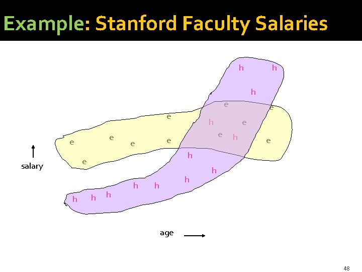
The CURE Algorithm �Problem with BFR/k-means: § Assumes clusters are normally distributed in each dimension. § And axes are fixed – ellipses at an angle are not OK. �CURE: § Assumes a Euclidean distance. § Allows clusters to assume any shape. 47

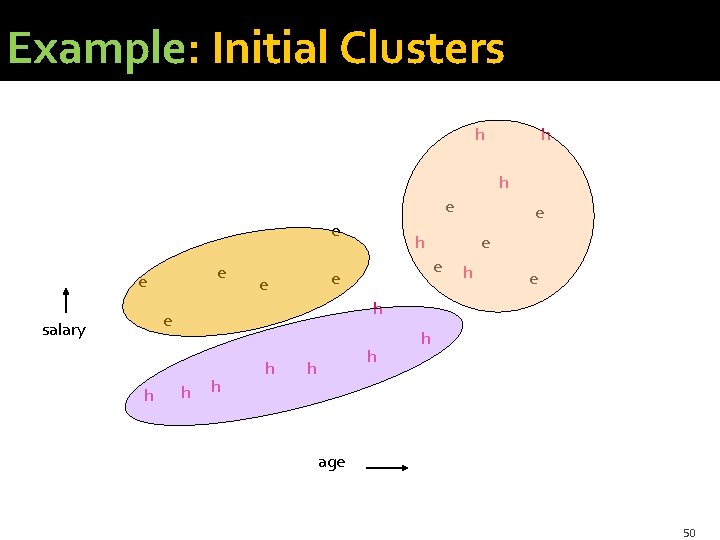
Example: Stanford Faculty Salaries h h h e e h e salary h e e e h h h age 48

Starting CURE Pick a random sample of points that fit in main memory. 2. Cluster these points hierarchically – group nearest points/clusters. 3. For each cluster, pick a sample of points, as dispersed as possible. 4. From the sample, pick representatives by moving them (say) 20% toward the centroid of the cluster. 1. 49

Example: Initial Clusters h h h e e h e salary h e e e h h h age 50

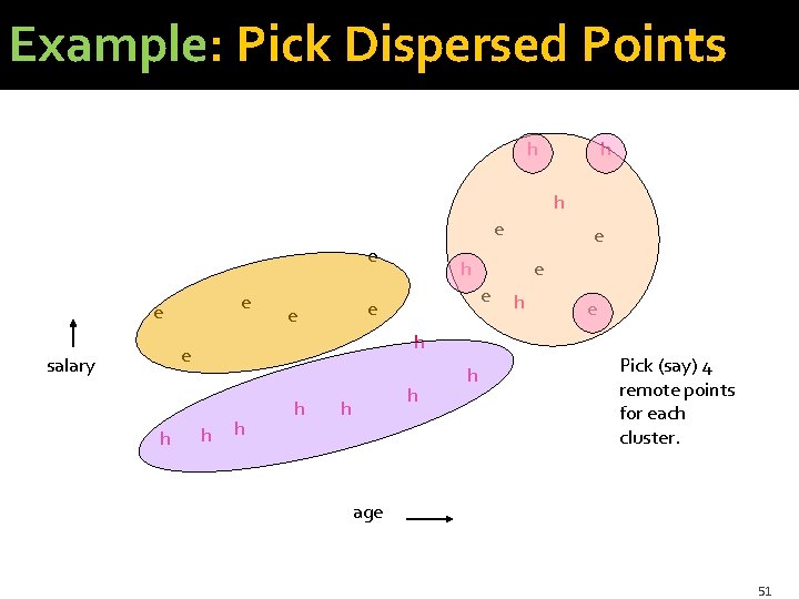
Example: Pick Dispersed Points h h h e e h e salary h e e e h h e Pick (say) 4 remote points for each cluster. age 51

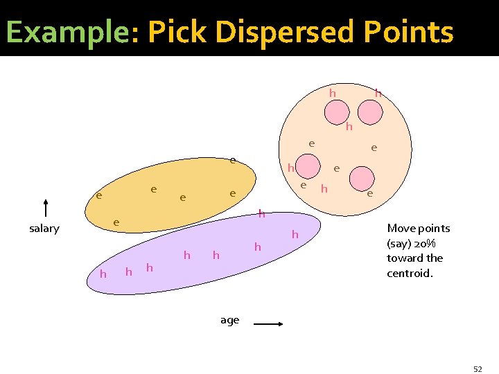
Example: Pick Dispersed Points h h h e e h e salary h e e e h h e Move points (say) 20% toward the centroid. age 52

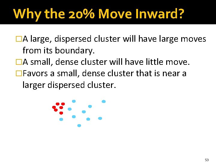
Why the 20% Move Inward? �A large, dispersed cluster will have large moves from its boundary. �A small, dense cluster will have little move. �Favors a small, dense cluster that is near a larger dispersed cluster. 53

Finishing CURE �Now, visit each point p in the data set. �Place it in the “closest cluster. ” § Normal definition of “closest”: that cluster with the closest (to p) among all the sample points of all the clusters. 54