Reinforcement Learning Chapter 21 Vassilis Athitsos Reinforcement Learning

Reinforcement Learning Chapter 21 Vassilis Athitsos

Reinforcement Learning • In previous chapters: – Learning from examples. • Reinforcement learning: – Learning what to do. • Learning to fly (a helicopter). • Learning to play a game. • Learning to walk. – Learning based on rewards.

Relation to MDPs • Feedback can be provided at the end of the sequence of actions, or more frequently. – Compare chess and ping-pong. • No complete model of environment. – Transitions may be unknown. • Reward function unknown.

Agents • Utility-based agent: – Learns utility function on states. • Q-learning agent: – Learns utility function on (action, state) pairs. • Reflex agent: – Learns function mapping states to actions.

Passive Reinforcement Learning • Assume fully observable environment. • Passive learning: – Policy is fixed (behavior does not change). – The agent learns how good each state is. • Similar to policy evaluation, but: – Transition function and reward function or unknown. • Why is it useful?

Passive Reinforcement Learning • Assume fully observable environment. • Passive learning: – Policy is fixed (behavior does not change). – The agent learns how good each state is. • Similar to policy evaluation, but: – Transition function and reward function or unknown. • Why is it useful? – For future policy revisions.

Direct Utility Estimation • For each state the agent ever visits: – For each time the agent visits the state: • Keep track of the accumulated rewards from the visit onwards. • Similar to inductive learning: – Learning a function on states using samples. • Weaknesses: – Ignores correlations between utilities of neighboring states. – Converges very slowly.

Adaptive Dynamic Programming • Learns transitions and state utilities. • Plugs values into Bellman equations. • Solves equations with linear algebra, or policy iteration. • Problem:

Adaptive Dynamic Programming • Learns transitions and state utilities. • Plugs values into Bellman equations. • Solves equations with linear algebra, or policy iteration. • Problem: – Intractable for large number of states. • Example: backgammon. – 1050 equations, with 1050 unknowns.

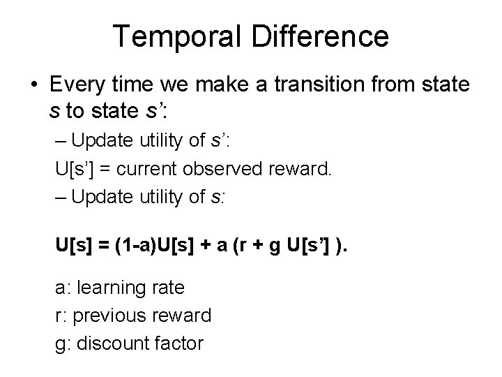
Temporal Difference • Every time we make a transition from state s to state s’: – Update utility of s’: U[s’] = current observed reward. – Update utility of s: U[s] = (1 -a)U[s] + a (r + g U[s’] ). a: learning rate r: previous reward g: discount factor

Properties of Temporal Difference • What happens when an unlikely transition occurs?

Properties of Temporal Difference • What happens when an unlikely transition occurs? – U[s] becomes a bad approximation of true utility. – However, U[s] is rarely a bad approximation. • Average value of U[s] converges to correct value. • If a decreases over time, U[s] converges to correct value.

Hybrid Methods • ADP: – More accurate, slower, intractable for large numbers of states. • TD: – Less accurate, faster, tractable. • An intermediate approach:

Hybrid Methods • ADP: – More accurate, slower, intractable for large numbers of states. • TD: – Less accurate, faster, tractable. • An intermediate approach: Pseudoexperiences: – Imagine transitions that have not happened. – Update utilities according to those transitions.

Hybrid Methods • Making ADP more efficient: – Do a limited number of adjustments after each transition. – Use estimated transition probabilities to identify the most useful adjustments.

Active Reinforcement Learning • Using passive reinforcement learning, utilities of states and transition probabilities are learned. • Those utilities and transitions can be plugged into Bellman equations. • Problem?

Active Reinforcement Learning • Using passive reinforcement learning, utilities of states and transition probabilities are learned. • Those utilities and transitions can be plugged into Bellman equations. • Problem? – Bellman equations give optimal solutions given correct utility and transition functions. – Passive reinforcement learning produces approximate estimates of those functions. • Solutions?

Exploration/Exploitation • The goal is to maximize utility. • However, utility function is only approximately known. • Dilemma: should the agent – Maximize utility based on current knowledge, or – Try to improve current knowledge.

Exploration/Exploitation • The goal is to maximize utility. • However, utility function is only approximately known. • Dilemma: should the agent – Maximize utility based on current knowledge, or – Try to improve current knowledge. • Answer: – A little of both.

Exploration Function • U[s] = R[s] + g max {f(Q(a, s), N(a, s))}. R[s]: current reward. g: discount factor. Q(a, s): estimated utility of performing action a in state s. N(a, s): number of times action a has been performed in state s. f(u, n): preference according to utility and degree of exploration so far for (a, s). • Initialization: U[s] = optimistically large value.

Q-learning • Learning utility of state-action pairs. U[s] = max Q(a, s). • Learning can be done using TD: Q(a, s) = (1 -b) Q(a, s) + b(R(s) + g max(Q(a’, s’)) b: learning factor g: discount factor s’: next state a’: possible action at next state

Generalization in Reinforcement Learning • How do we apply reinforcement learning problems with huge numbers of states (chess, backgammon, …)?

Generalization in Reinforcement Learning • How do we apply reinforcement learning problems with huge numbers of states (chess, backgammon, …)? • Solution similar to estimating probabilities of a huge number of events:

Generalization in Reinforcement Learning • How do we apply reinforcement learning problems with huge numbers of states (chess, backgammon, …)? • Solution similar to estimating probabilities of a huge number of events: – Learn parametric functions, where parameters are features of each state. • Example: chess. – 20 features adequate for describing the current board.

Learning Parametric Utility Functions For Backgammon • First approach: – Design weighted linear functions of 16 terms. – Collect training set of board states. – Ask human experts to evaluate training states. • Result: – Program not competitive with human experts. – Collecting training data was very tedious.

Learning Parametric Utility Functions For Backgammon • Second approach: – Design weighted linear functions of 16 terms. – Let the system play against itself. – Reward provided at the end of each game. • Result (after 300, 000 games, a few weeks): – Program competitive with best players in the world.