Reinforcement Learning CSE 4309 Machine Learning Vassilis Athitsos

Reinforcement Learning CSE 4309 – Machine Learning Vassilis Athitsos Computer Science and Engineering Department University of Texas at Arlington 1

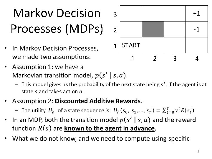
Markov Decision Processes (MDPs) 3 +1 2 -1 1 START 1 2 3 4 2

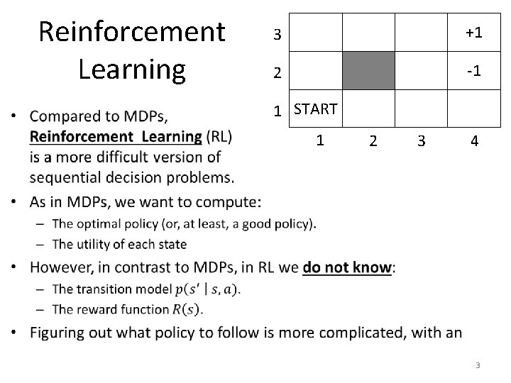
Reinforcement Learning 3 +1 2 -1 1 START 1 2 3 4 3

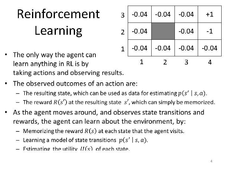
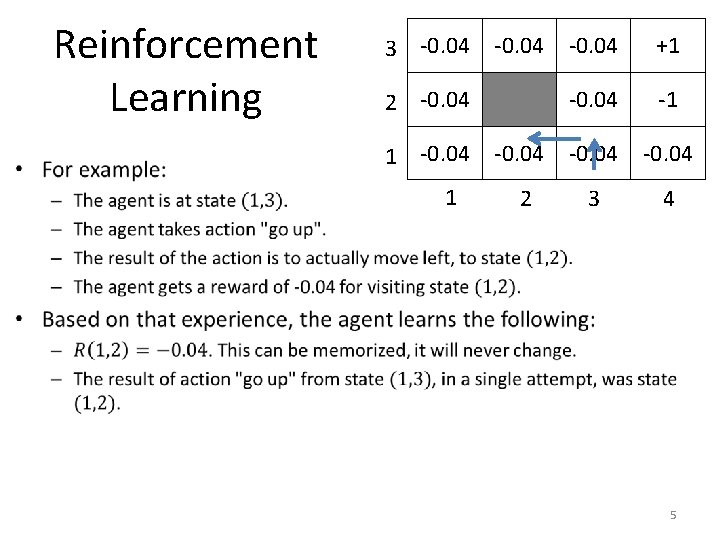
Reinforcement Learning 3 -0. 04 +1 -0. 04 2 3 4 2 -0. 04 1 4

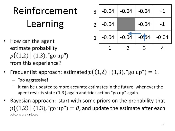
Reinforcement Learning 3 -0. 04 +1 -0. 04 2 3 4 2 -0. 04 1 5

Reinforcement Learning 3 -0. 04 +1 -0. 04 2 3 4 2 -0. 04 1 6

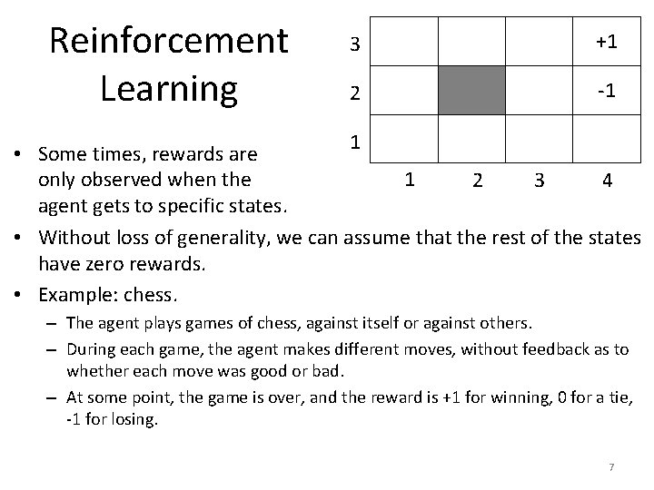
Reinforcement Learning 3 +1 2 -1 1 • Some times, rewards are only observed when the 1 2 3 4 agent gets to specific states. • Without loss of generality, we can assume that the rest of the states have zero rewards. • Example: chess. – The agent plays games of chess, against itself or against others. – During each game, the agent makes different moves, without feedback as to whether each move was good or bad. – At some point, the game is over, and the reward is +1 for winning, 0 for a tie, -1 for losing. 7

Reinforcement Learning vs. Supervised Learning • Learning to play chess can be approached as a reinforcement learning problem, or as a supervised learning problem. • Reinforcement learning approach: – The agent plays games of chess, against itself or against others. – During each game, the agent makes different moves, without feedback as to whether each move was good or bad. – At some point, the game is over, and the reward is +1 for winning, 0 for a tie, -1 for losing. • Supervised learning approach: – The agent plays games of chess, against itself or against others. – During each game, the agent makes different moves. – For every move, an expert provides an evaluation of that move. • Pros and cons of each approach? 8

Reinforcement Learning vs. Supervised Learning • In the chess example, the big advantage of reinforcement learning is that no effort is required from human experts to evaluate moves. – Lots of training data can be generated by having the agent play against itself or other artificial agents. – No human time is spent. • Supervised learning requires significant human effort. – If that effort can be spared, supervised learning has more information, and thus should learn a better strategy. – However, in many sequential decision problems, the state space is so large, that it is infeasible for humans to evaluate a sufficiently large number of states. 9

Passive and Active RL • In typical RL problems, the agent proceeds step-by-step, where every step involves: – Deciding what action to take, based on its current policy. – Taking the action, observing the outcome, and modifying accordingly its current policy. • This problem is called active reinforcement learning, and we will look at some methods for solving it. • However, first, we will study an easier RL problem, called passive reinforcement learning. • In this easier version: – The policy is fixed. – The transition model and reward function are still unknown. – The goal is simply to compute the utility value of each state. 10

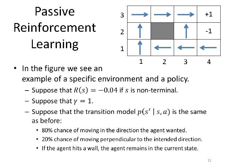
Passive Reinforcement Learning • 3 +1 2 -1 1 1 2 3 4 11

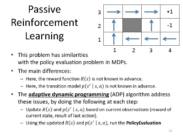
Passive Reinforcement Learning • 3 +1 2 -1 1 1 2 3 4 12

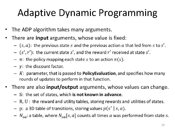
Adaptive Dynamic Programming • 13

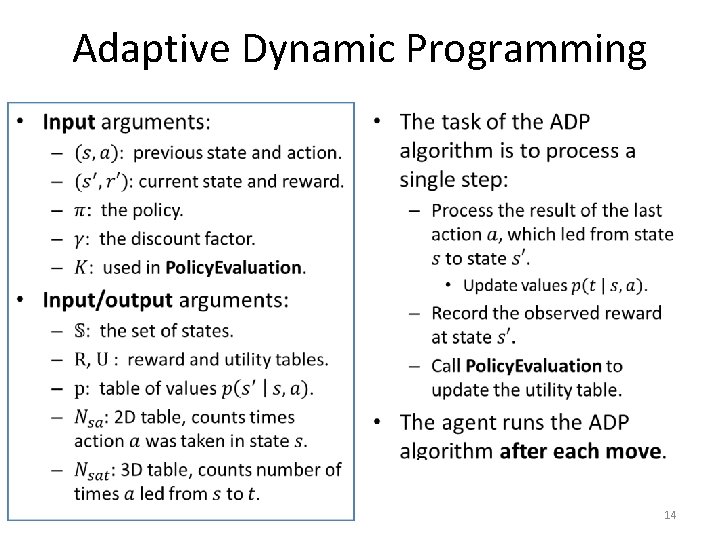
Adaptive Dynamic Programming • • 14

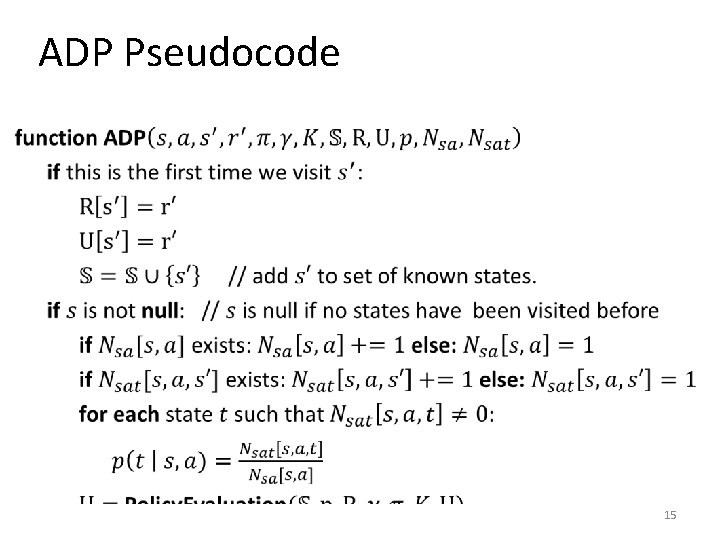
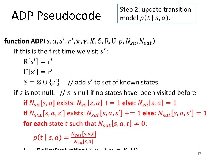
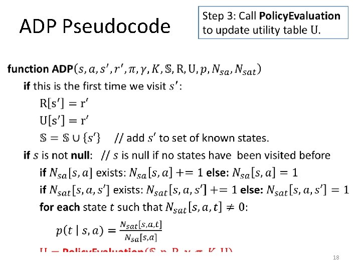
ADP Pseudocode • 15

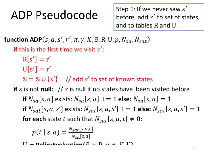
ADP Pseudocode • 16

ADP Pseudocode • 17

ADP Pseudocode • 18

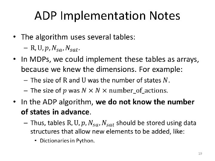
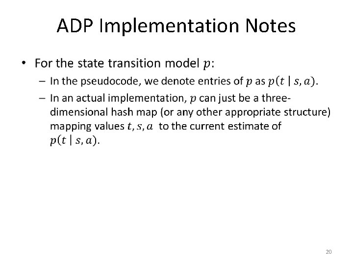
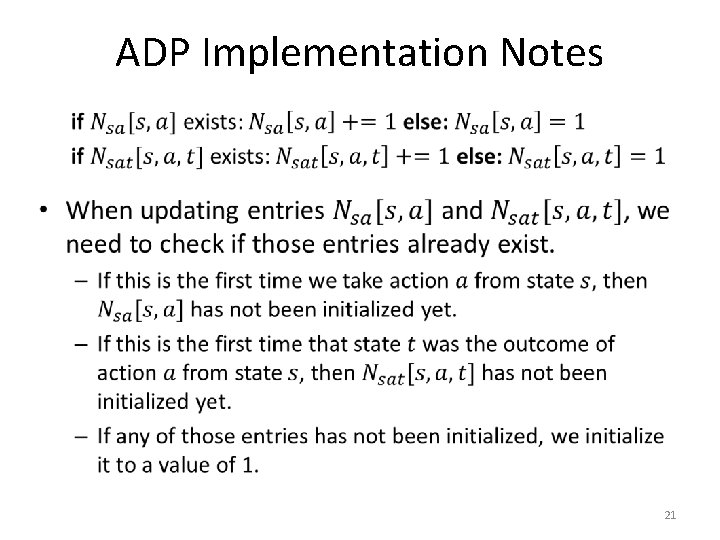
ADP Implementation Notes • 19

ADP Implementation Notes • 20

ADP Implementation Notes • 21

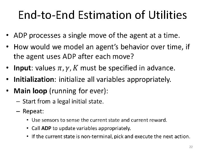
End-to-End Estimation of Utilities • 22

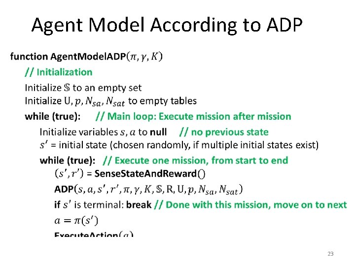
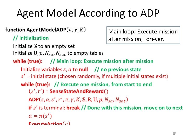
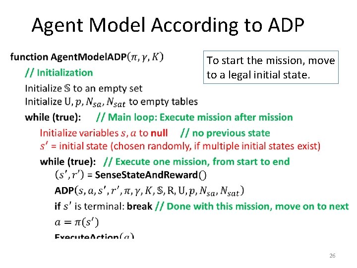
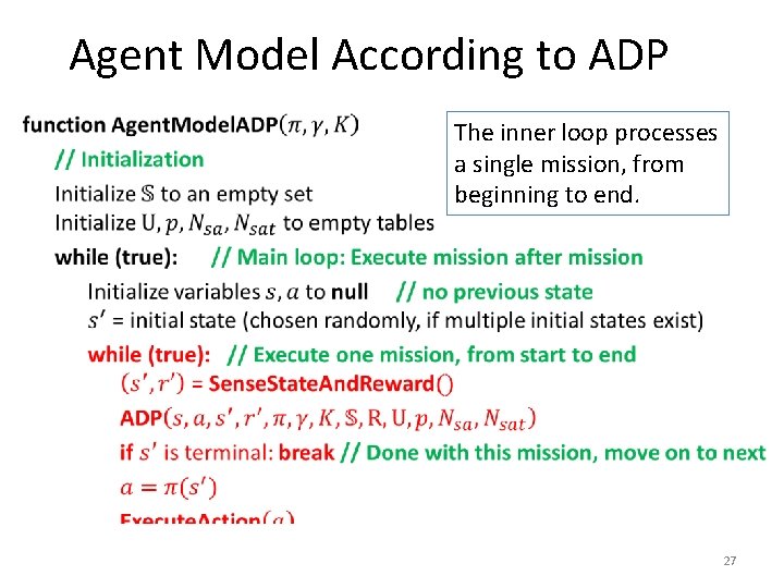
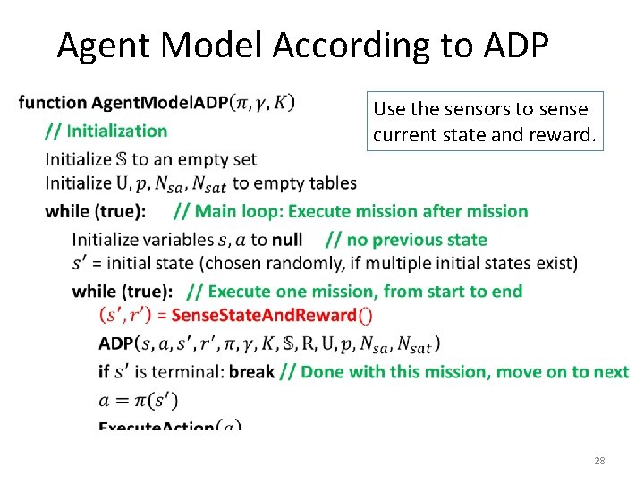
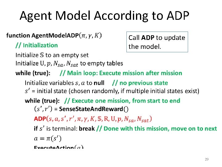
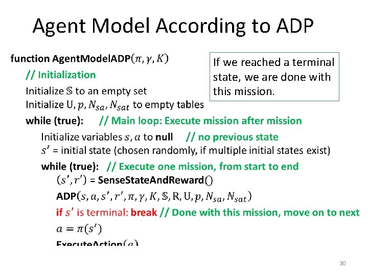
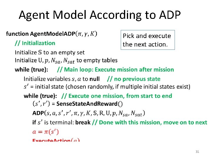
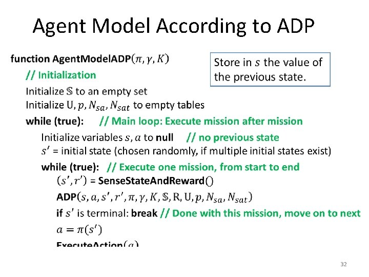
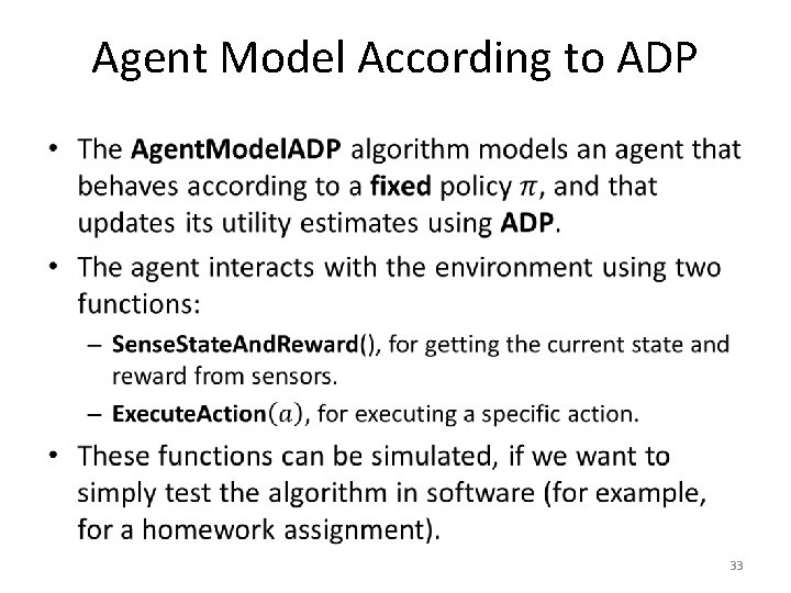
Agent Model According to ADP • 23

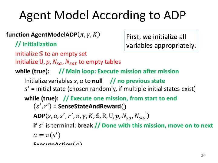
Agent Model According to ADP • First, we initialize all variables appropriately. 24

Agent Model According to ADP • Main loop: Execute mission after mission, forever. 25

Agent Model According to ADP • To start the mission, move to a legal initial state. 26

Agent Model According to ADP • The inner loop processes a single mission, from beginning to end. 27

Agent Model According to ADP • Use the sensors to sense current state and reward. 28

Agent Model According to ADP • Call ADP to update the model. 29

Agent Model According to ADP • If we reached a terminal state, we are done with this mission. 30

Agent Model According to ADP • Pick and execute the next action. 31

Agent Model According to ADP • 32

Agent Model According to ADP • 33

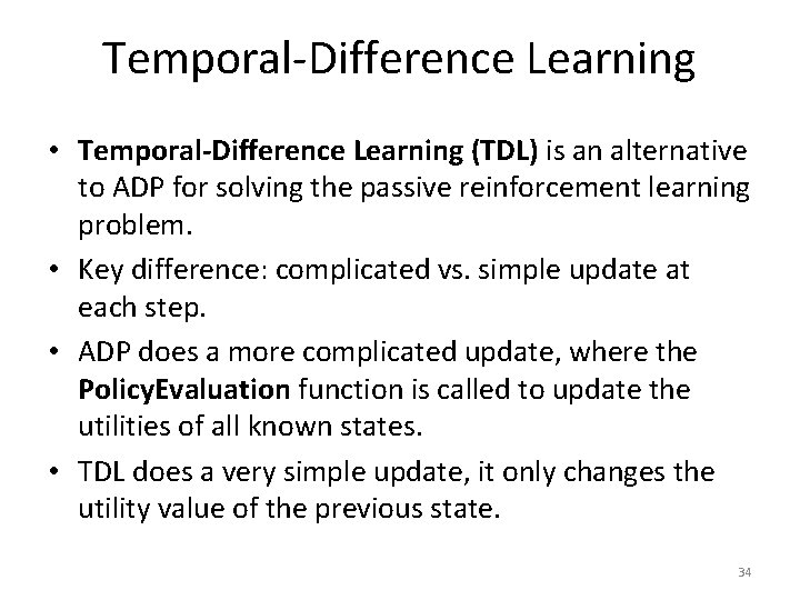
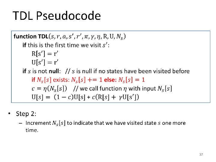
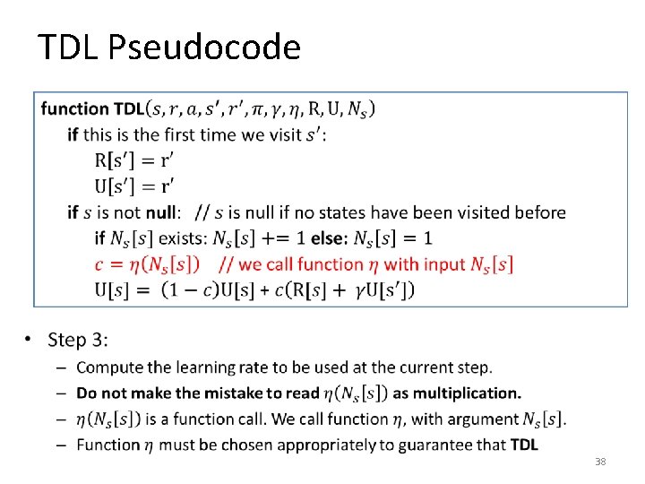
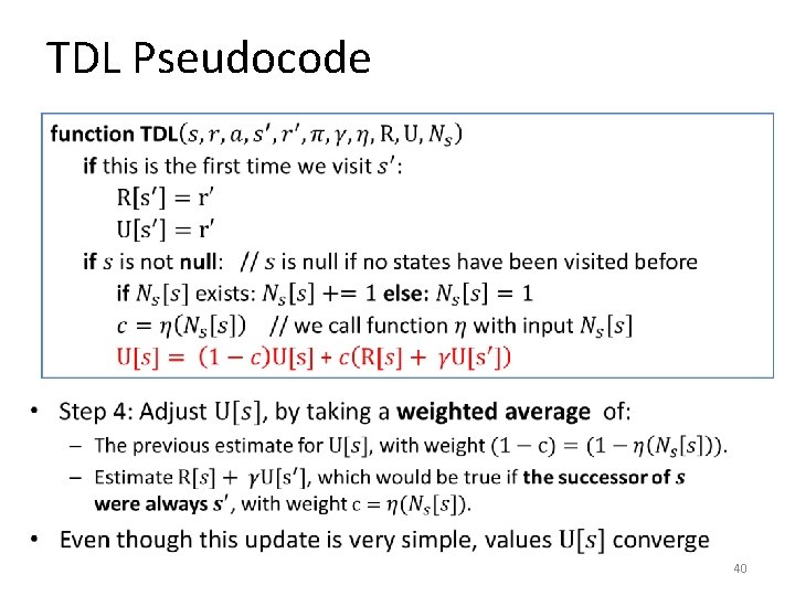
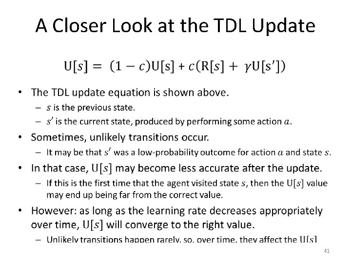
Temporal-Difference Learning • Temporal-Difference Learning (TDL) is an alternative to ADP for solving the passive reinforcement learning problem. • Key difference: complicated vs. simple update at each step. • ADP does a more complicated update, where the Policy. Evaluation function is called to update the utilities of all known states. • TDL does a very simple update, it only changes the utility value of the previous state. 34

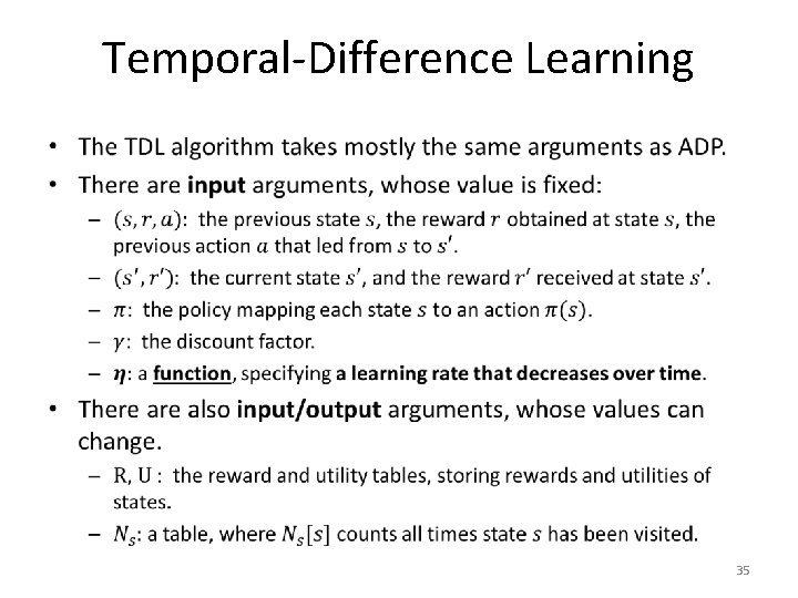
Temporal-Difference Learning • 35

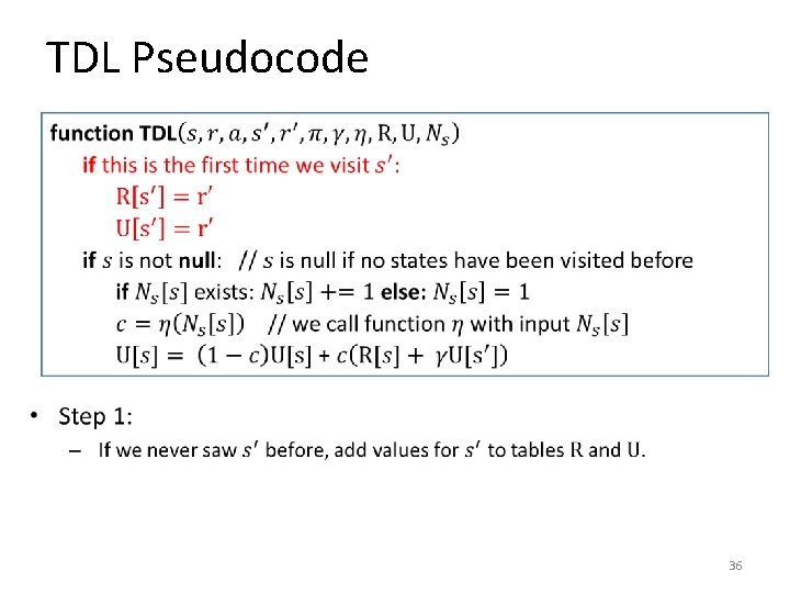
TDL Pseudocode • 36

TDL Pseudocode • 37

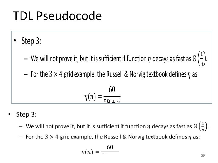
TDL Pseudocode • 38

TDL Pseudocode • 39

TDL Pseudocode • 40

A Closer Look at the TDL Update • 41

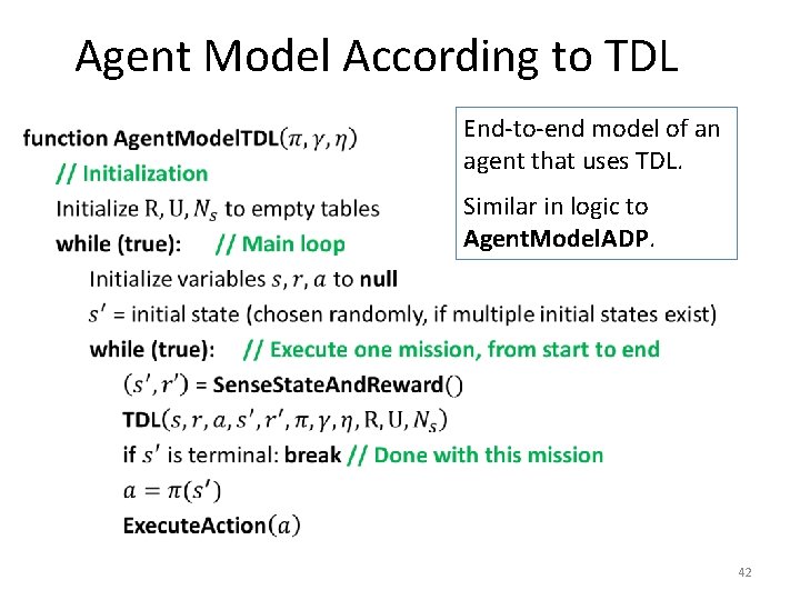
Agent Model According to TDL • End-to-end model of an agent that uses TDL. Similar in logic to Agent. Model. ADP. 42

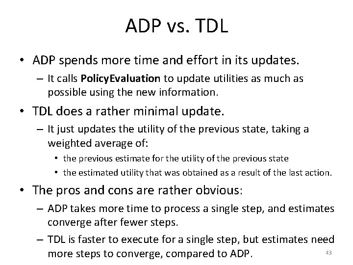
ADP vs. TDL • ADP spends more time and effort in its updates. – It calls Policy. Evaluation to update utilities as much as possible using the new information. • TDL does a rather minimal update. – It just updates the utility of the previous state, taking a weighted average of: • the previous estimate for the utility of the previous state • the estimated utility that was obtained as a result of the last action. • The pros and cons are rather obvious: – ADP takes more time to process a single step, and estimates converge after fewer steps. – TDL is faster to execute for a single step, but estimates need 43 more steps to converge, compared to ADP.

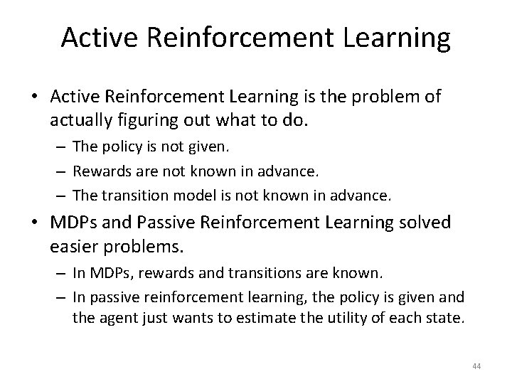
Active Reinforcement Learning • Active Reinforcement Learning is the problem of actually figuring out what to do. – The policy is not given. – Rewards are not known in advance. – The transition model is not known in advance. • MDPs and Passive Reinforcement Learning solved easier problems. – In MDPs, rewards and transitions are known. – In passive reinforcement learning, the policy is given and the agent just wants to estimate the utility of each state. 44

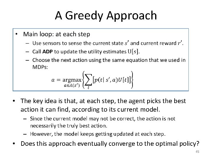
A Greedy Approach • The key idea is that, at each step, the agent picks the best action it can find, according to its current model. – Since the current model may not be correct, the action is not necessarily the truly best action. – However, the model keeps getting updated at each step. • Does this approach eventually converge to the optimal policy? 45

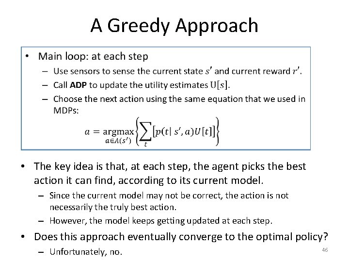
A Greedy Approach • The key idea is that, at each step, the agent picks the best action it can find, according to its current model. – Since the current model may not be correct, the action is not necessarily the truly best action. – However, the model keeps getting updated at each step. • Does this approach eventually converge to the optimal policy? – Unfortunately, no. 46

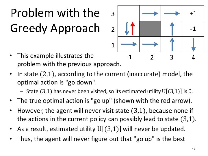
Problem with the Greedy Approach 3 +1 2 -1 1 • 1 2 3 4 47

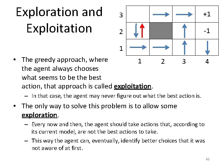
Exploration and Exploitation 3 +1 2 -1 1 • The greedy approach, where 1 the agent always chooses what seems to be the best action, that approach is called exploitation. 2 3 4 – In that case, the agent may never figure out what the best action is. • The only way to solve this problem is to allow some exploration. – Every now and then, the agent should take actions that, according to its current model, are not the best actions to take. – This way the agent can, eventually, identify better choices that it was not aware of at first. 48

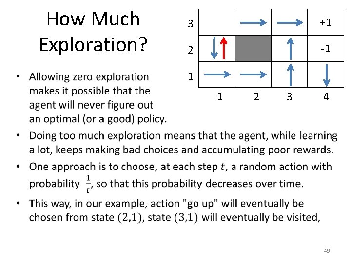
How Much Exploration? • 3 +1 2 -1 1 1 2 3 4 49

How Much Exploration? • 3 +1 2 -1 1 1 2 3 4 50

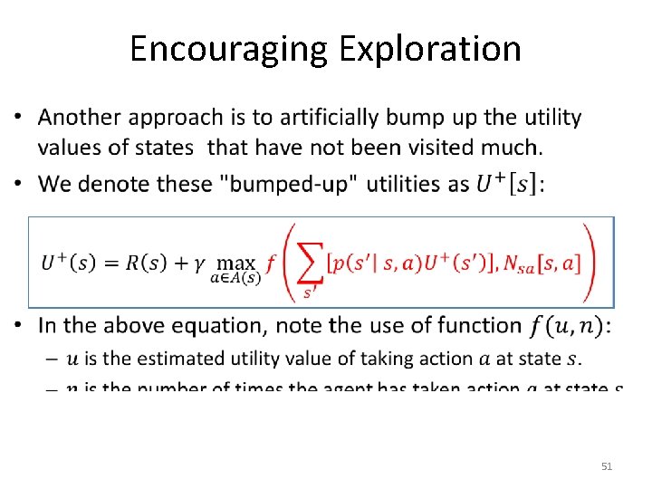
Encouraging Exploration • 51

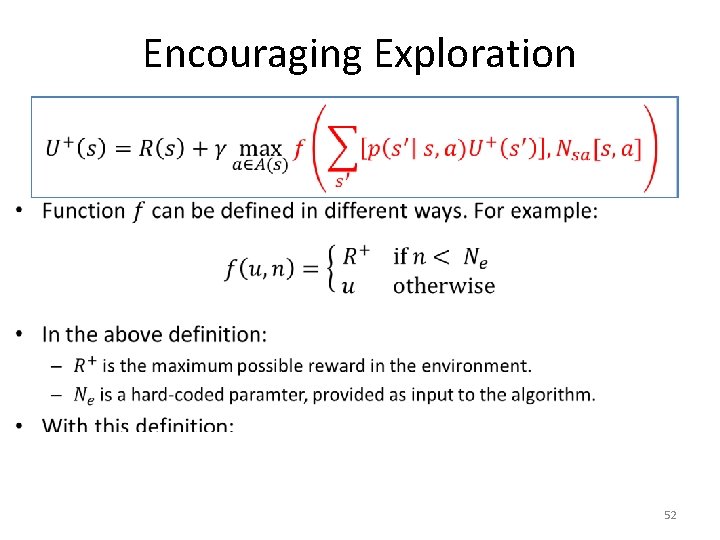
Encouraging Exploration • 52

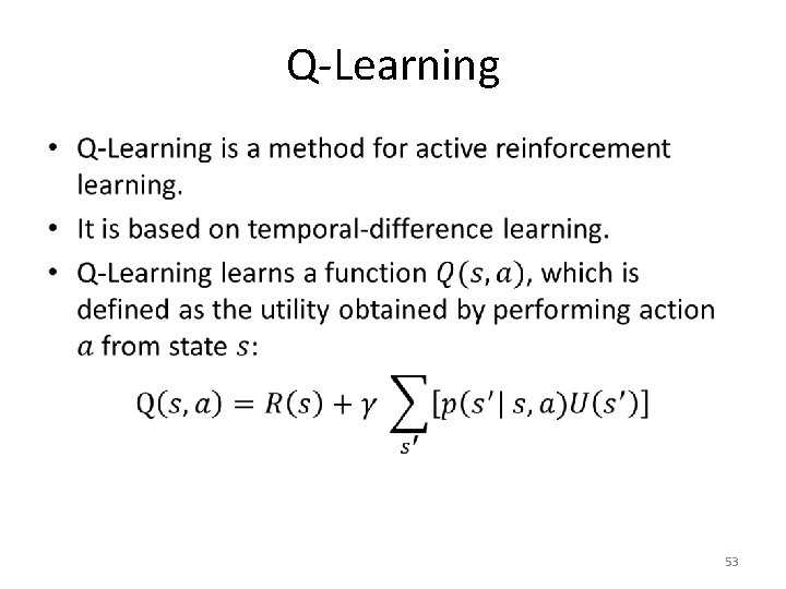
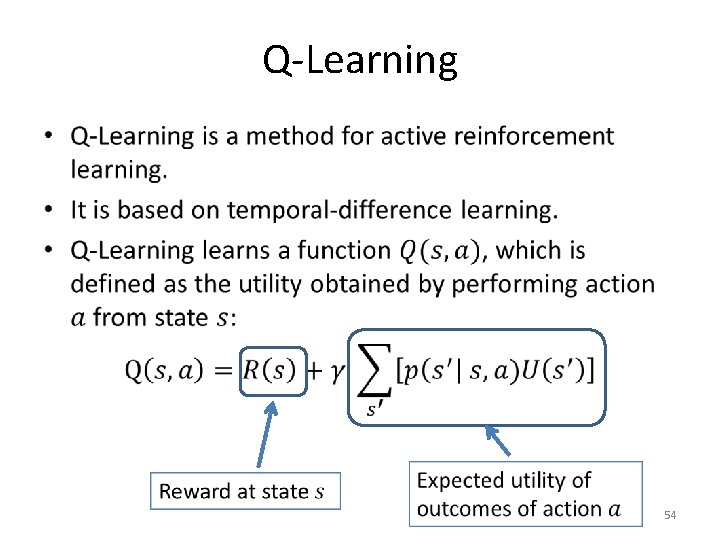
Q-Learning • 53

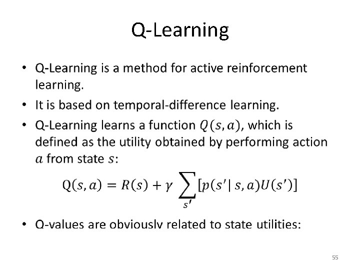
Q-Learning • 54

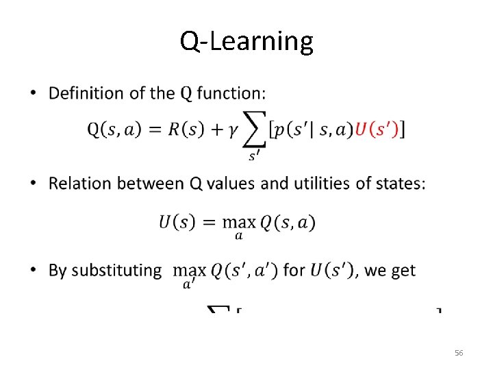
Q-Learning • 55

Q-Learning • 56

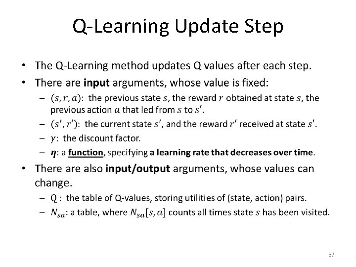
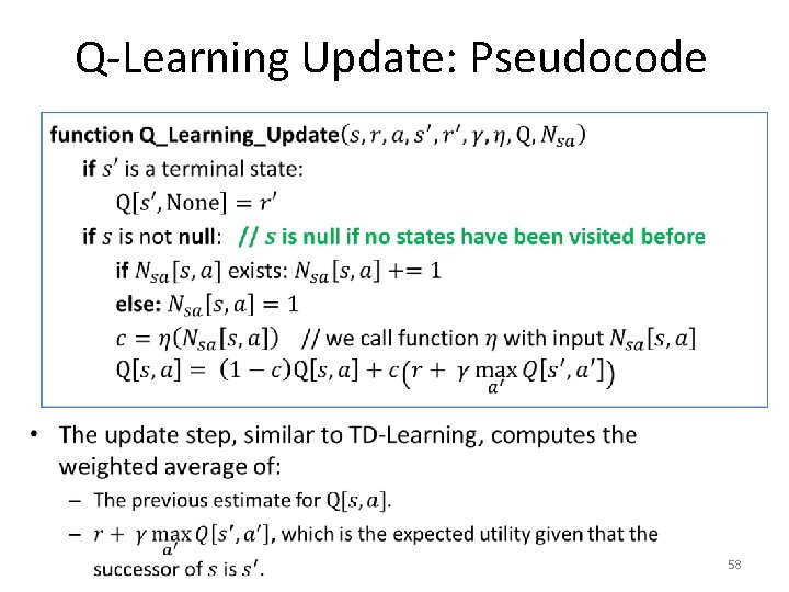
Q-Learning Update Step • 57

Q-Learning Update: Pseudocode • 58

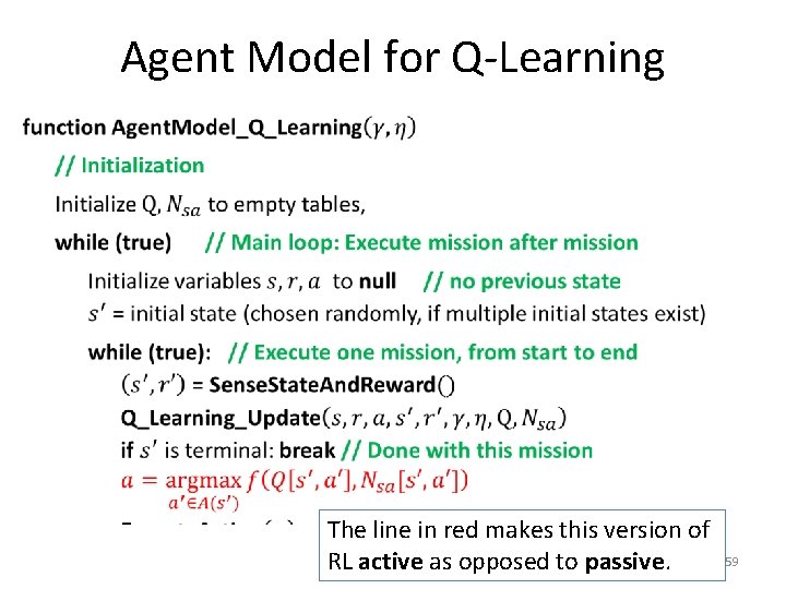
Agent Model for Q-Learning • The line in red makes this version of RL active as opposed to passive. 59

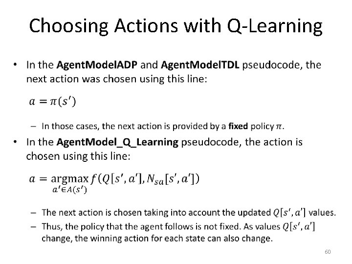
Choosing Actions with Q-Learning • 60

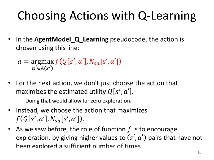
Choosing Actions with Q-Learning • 61

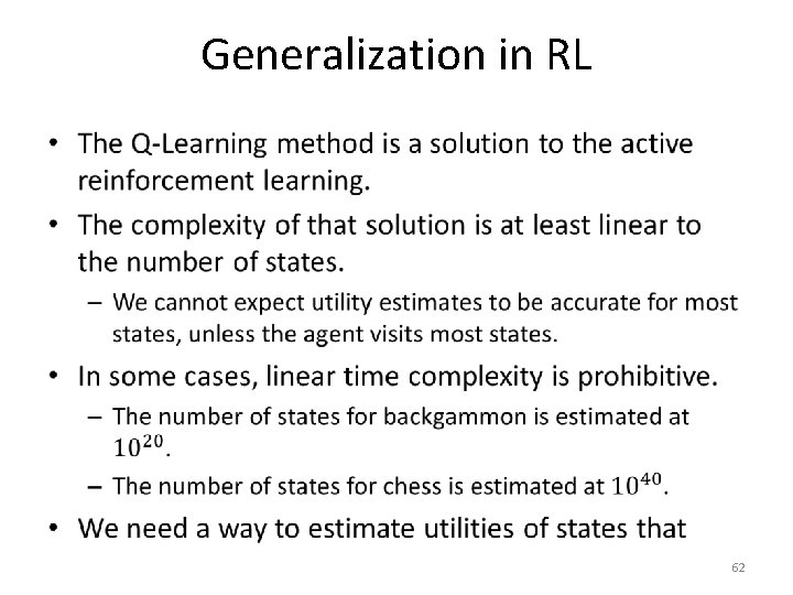
Generalization in RL • 62

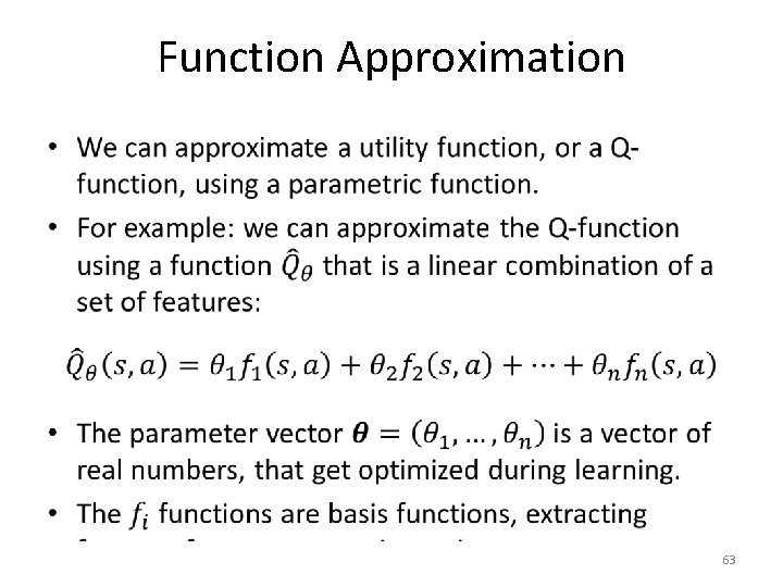
Function Approximation • 63

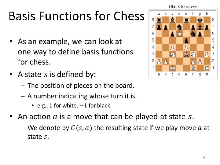
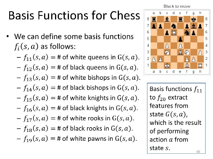
Basis Functions for Chess • 64

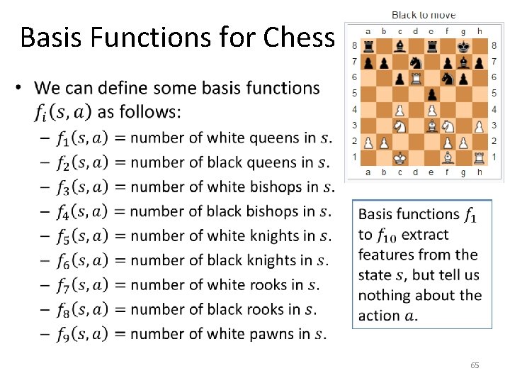
Basis Functions for Chess • 65

Basis Functions for Chess • 66

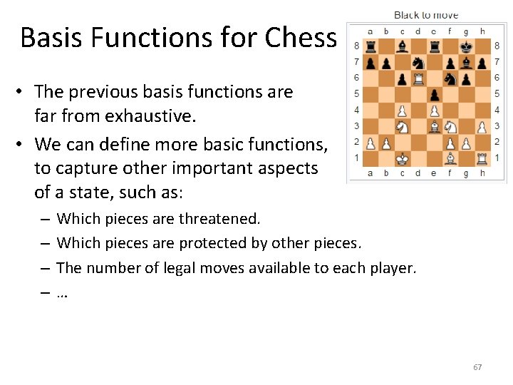
Basis Functions for Chess • The previous basis functions are far from exhaustive. • We can define more basic functions, to capture other important aspects of a state, such as: – – Which pieces are threatened. Which pieces are protected by other pieces. The number of legal moves available to each player. … 67

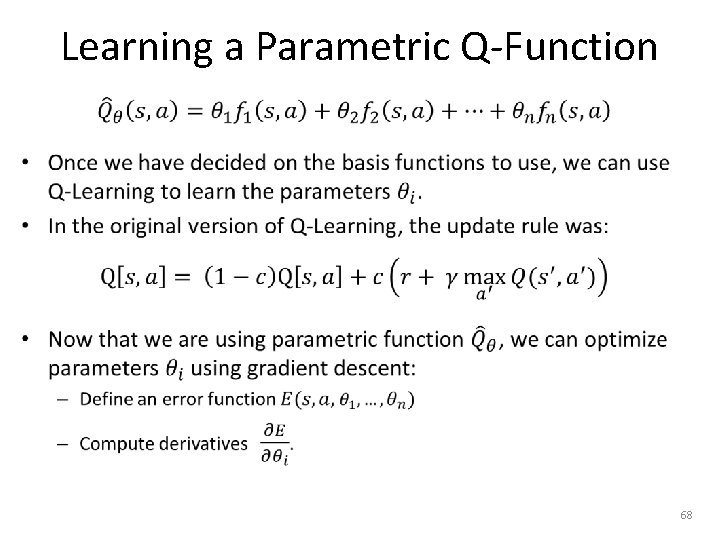
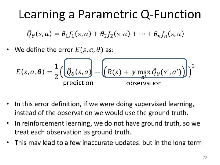
Learning a Parametric Q-Function • 68

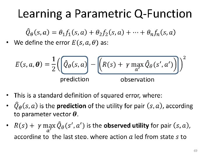
Learning a Parametric Q-Function • prediction observation 69

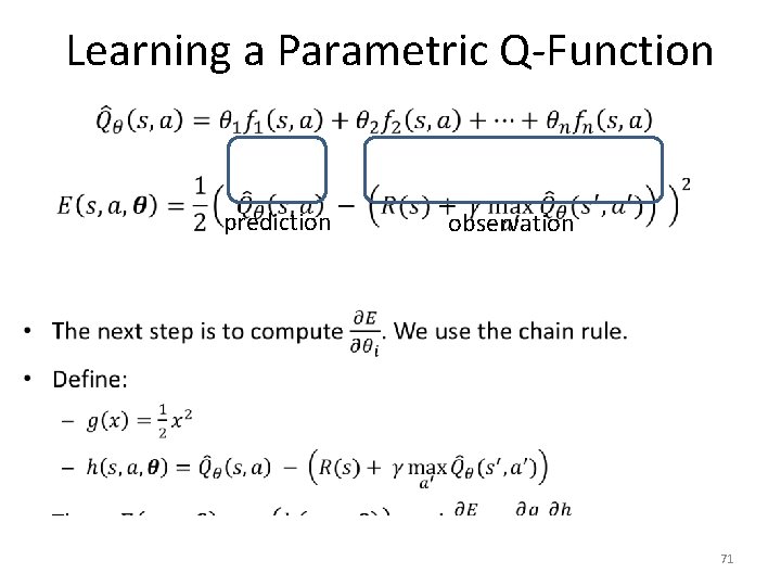
Learning a Parametric Q-Function • prediction observation 70

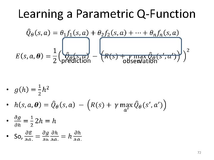
Learning a Parametric Q-Function • prediction observation 71

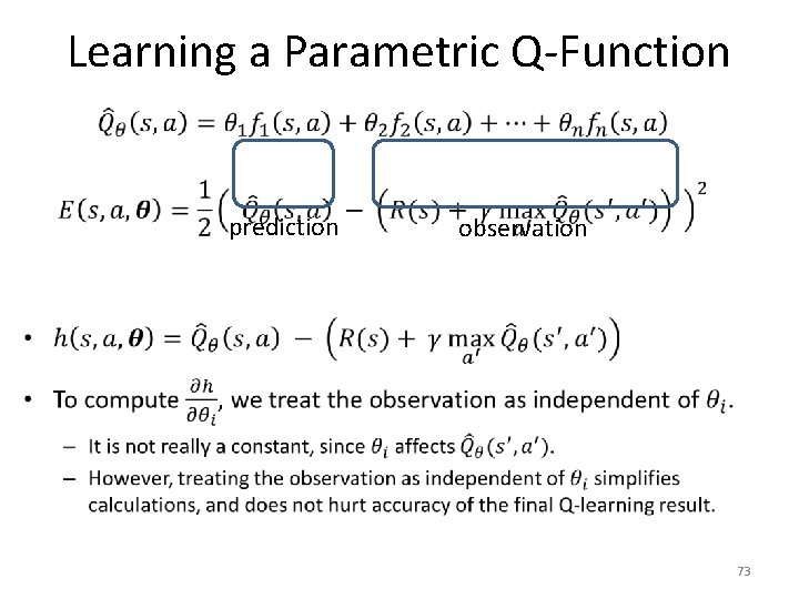
Learning a Parametric Q-Function • prediction observation 72

Learning a Parametric Q-Function • prediction observation 73

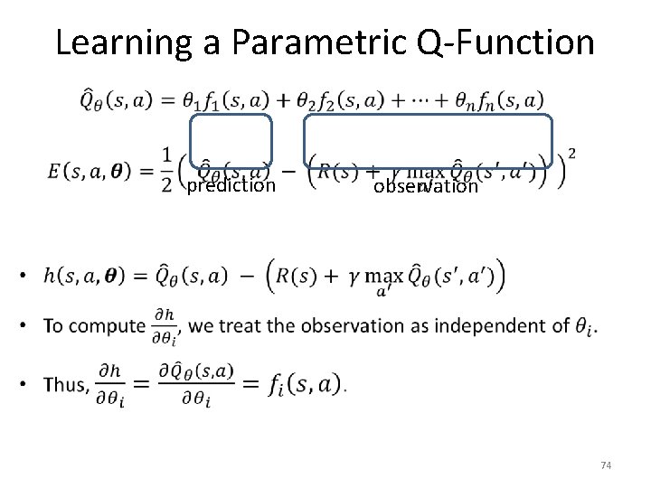
Learning a Parametric Q-Function • prediction observation 74

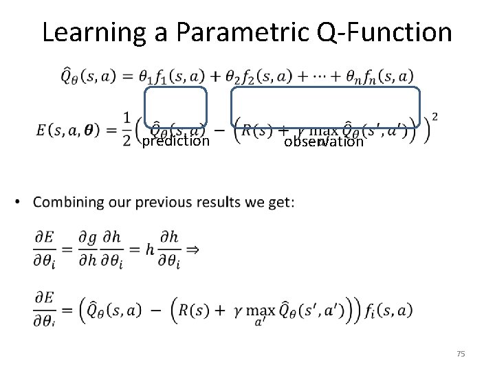
Learning a Parametric Q-Function • prediction observation 75

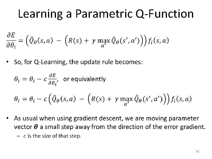
Learning a Parametric Q-Function • 76

Reinforcement Learning - Recap • 77

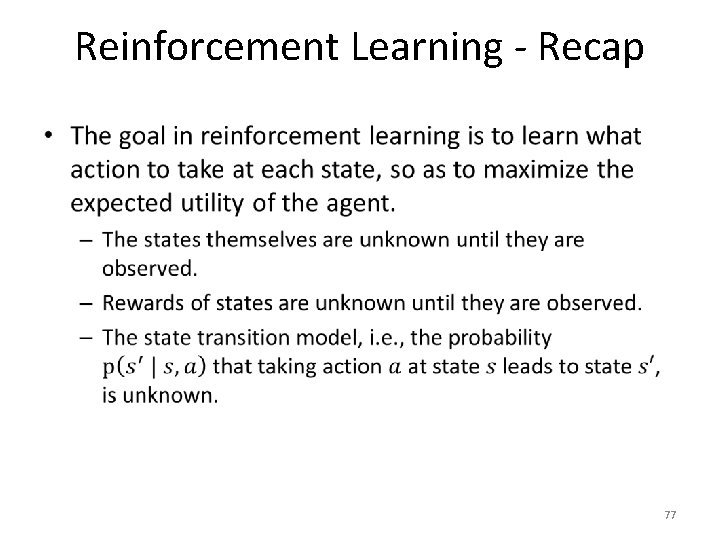
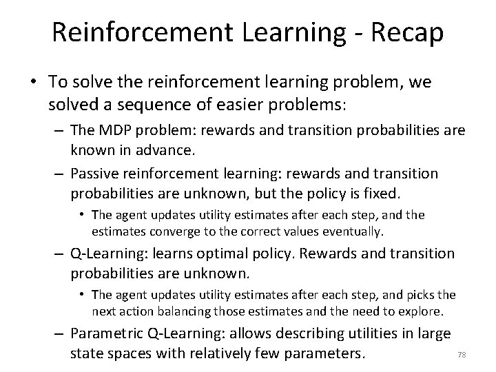
Reinforcement Learning - Recap • To solve the reinforcement learning problem, we solved a sequence of easier problems: – The MDP problem: rewards and transition probabilities are known in advance. – Passive reinforcement learning: rewards and transition probabilities are unknown, but the policy is fixed. • The agent updates utility estimates after each step, and the estimates converge to the correct values eventually. – Q-Learning: learns optimal policy. Rewards and transition probabilities are unknown. • The agent updates utility estimates after each step, and picks the next action balancing those estimates and the need to explore. – Parametric Q-Learning: allows describing utilities in large 78 state spaces with relatively few parameters.