CH 18 Reinforcement Learning 18 1 Introduction Kinds

CH. 18: Reinforcement Learning 18. 1 Introduction Kinds of learning: 1. Supervised learning, 2. 2. Unsupervised learning, 3. Semi-supervised learning -- learning using labeled and unlabeled examples, learning via hints, indirect answers, etc. . 4. Reinforcement learning -- learning via continuously interacting with environment; We focus on reinforcement learning (RL). 1

Potential applications of RL 2

18. 2 Elements of RL The agent (learner) takes an action; the environment changes its state; the agent receives immediately or later a reward from the environment. The goal is to find an optimal policy that maximizes the cumulated reward. 2

4 Example 1: Chess-playing i) Agent: player ii) Environment: chess board iii) Action: move, iv) State: locations of the board each of which is either empty or with a chessman v) Reward: the feedback is at the end of the game vi) Goal: win a game through a sequence of move. 3

5 Example 2: Robot navigation i) Agent: robot ii) Environment: room iii) Action: move iv) State: grid at which the robot locates v) Reward: the feedback after a move vi) Goal: reach the goal state with the maximum cumulative reward. 4

Let S: a set of states of the environment A: a set of actions feasible for the agent At time t, current state, present action, policy stationary policy: nonstationary policy: time varying reward function, state transition function 5

Define value function i. e. , the cumulative reward from state following policy. Alternatives of value function: Finite horizon reward: Infinite horizon reward: Average reward: Discounted reward: discount factor 5

Objective: Find optimal policy optimal cumulative reward Optimal action: 7

Example: Actions: Discount factor: 8

9

10

Likewise: 11

18. 3 Q learning -- For learning the optimal policy based on Q values. Define i. e. , Q value is the reward received immediately upon executing a in s, plus the discounted cumulative value of following the optimal policy. Optimal action: 12

Optimal cumulative reward: ( recurrent formulation) Why Q rather than : The learner can acquire the optimal policy learning Q or . However, learning precise to know perfect knowledge of r and by needs while good Q can be iteratively learned via approximate or even without knowledge of r and . 13

Algorithm: 3. Repeat Step 2. On-policy: the policy is used to determine the next action. Off-policy: all actions are examined without using the policy. 14

SARSA algorithm – On-policy Q learning 15

Example – Off-policy Q learning 16

The optimal policy: corresponds to selecting actions with maximal Q values. 17

18. 4 Temporal Difference (TD) Learning 1 9 Q learning iteratively reduces the discrepancy between Q values for adjacent states. TD learning reduces the discrepancy between Q values at different times. learning One-step lookahead value: Two-step lookahead value: 18

n-step lookahead value: 2 0 Combination : Recursive equivalence: 19

18. 5 Different Settings of RL 1. Actions may have deterministic or nondeterministic (stochastic) outcomes (including reward and next state). 2. The agent may choose exploitation or exploration of states and actions. 3. Actions may have immediate or delayed rewards. 4. The agent may have complete (environment) or partial (agent) state. * Different settings lead to different definitions of V and Q functions. 20

-- For any state-action pair , a single reward

Model-based agent has built an Markov decision process (MDP). MDP is different from Markov chain (MC). MC 22

The expected values of V and Q are considered. Optimal action: 23

Policy Iteration Algorithm -- Use optimal action to find the optimal policy 24

(Bellman’s equation) Value Iteration Algorithm -- Use the optimal to find the optimal policy 25

18. 5. 3 Exploration/Exploitation Strategies Exploration of unknown states and actions to gather new information Exploitation of learned states and actions to maximize the cumulative reward ε-greedy search: Explore – with probability ε choose uniformly one action among all possible actions. Exploit – with probability 1 -ε choose the best action. Start with a high ε and gradually decrease it in order to initiate exploitation once enough exploration. 26

2 8 Probabilistic search: Choose action a according to probability Move from exploration to exploitation using Start with a large T and gradually decrease it. T large, T small, better actions exploration exploitation. 27

18. 5. 4 Partially Observable States (POS) 2 9 -- After taking an action at , the new state st+1 is not known exactly. An observation ot+1 is provided by sensors for inferring the state. The agent is endowed with a state estimator (SE) that produces belief (agent) state bt+1 based on i) last action at, ii) current observation ot+1, and iii) previous belief state bt. 28

A policy 3 0 generates the next action at based on bt+1. Q learning for POS: 29

Example: Tiger negative reward Treasure positive reward Let : probabilities that the tiger is in rooms Rewards: 30

No observation - The expected rewards of actions: 3 2 31

3 3 Partial observation I - A sensor with small negative reward is used to detect tiger’s presence o (observation), where : sensing action. Suppose the reliability of the sensor is specified by the probability of 0. 7 to detect tiger’s presence. 32

The belief in tiger’s position (Bay’s rule): 3 4 33

If we sense o. L, the expected rewards for the actions: 34

If we sense o. R, the expected rewards for the actions: 3 6 35

3 7 36

Partial observation II - Suppose there is a door (hidden state) between the two rooms and the tiger can move from one room to the other with probability = 0. 8 37

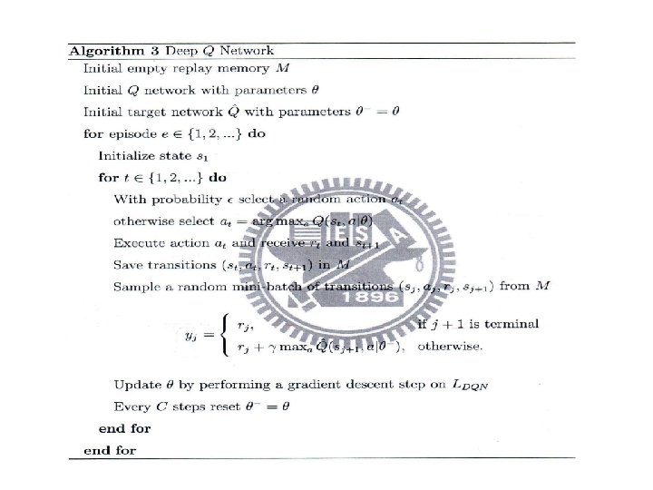
Deep Reinforcement Learning (DRL) -- Reinforcement learning + Deep learning Deep Q Networks (DQN) -- Uses a regression deep neural network (DNN), whose inputs: states + Q values -- Q learning: Loss function: In addition to DNN, DQN includes replay memory and target network Multiple Target Prediction for Deep Reinforcement Learning, National Chiao Tung University

• Replay memory: Every time the agent interacts with the environment, it saves the transition into the replay memory. When reaching the updating step, the agent randomly samples a mini-batch of transitions to train the network. • Target network (or Q network ): for accurately calculating Q values Loss function: The parameters of Q network are copied to target network every a few steps.

Double DQN Q-learning: Dueling Network Architectures -- State value function + state dependent action advantage function The state dependent action advantage function: where : the state-action value function : the state value function

Prioritized Experience Replay -- Marks data in replay memory with priority according to TD error The probability of sampling experience i To avoid bias resulting from non-uniform sampling, weighted-importance sampling is used. The weights are

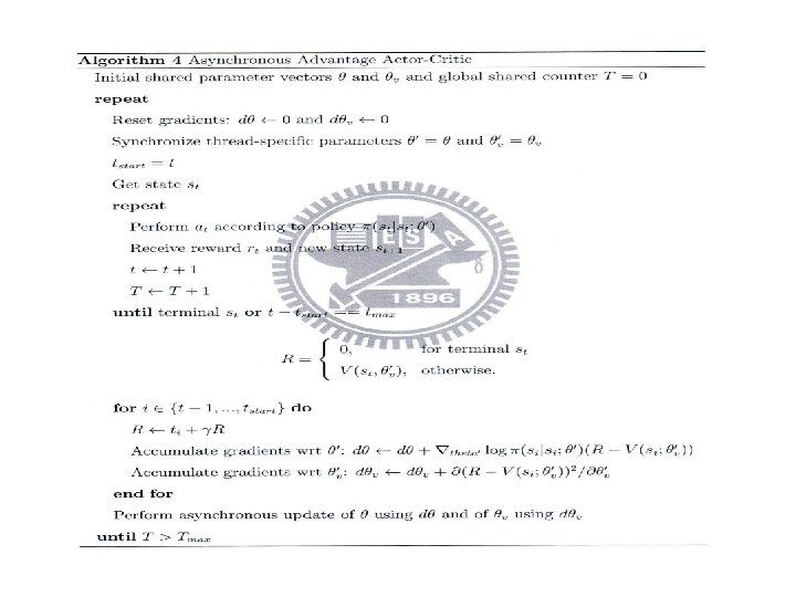
Asynchronous Advantage Actor-Critic -- The agent can interact with multiple environments at a time A policy and a value function are maintained. They are updated every actions. Updates:

Deep Deterministic Policy Gradient

Recent Researches in DRL Bootstrapped Deep Q Network

Hindsight Experience Replay

Continuous Q-Learning with NAF

Imagination Rollouts with Fitted Dynamics and i. LQG Exploration

Reference P. Y. Hung and J. T. chien, “Multiple Target Prediction for Deep Reinforcement Learning, ” Master Thesis, Institute of Communication Engineering, College of Electrical and Computer Engineering, National Chiao Tung University, Sep. 2017.