Reinforcement Learning Reinforcement Learning Agent State s Reward

Reinforcement Learning

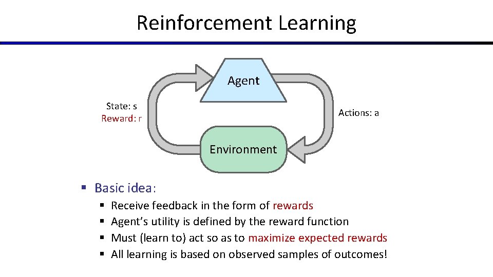
Reinforcement Learning Agent State: s Reward: r Actions: a Environment § Basic idea: § § Receive feedback in the form of rewards Agent’s utility is defined by the reward function Must (learn to) act so as to maximize expected rewards All learning is based on observed samples of outcomes!

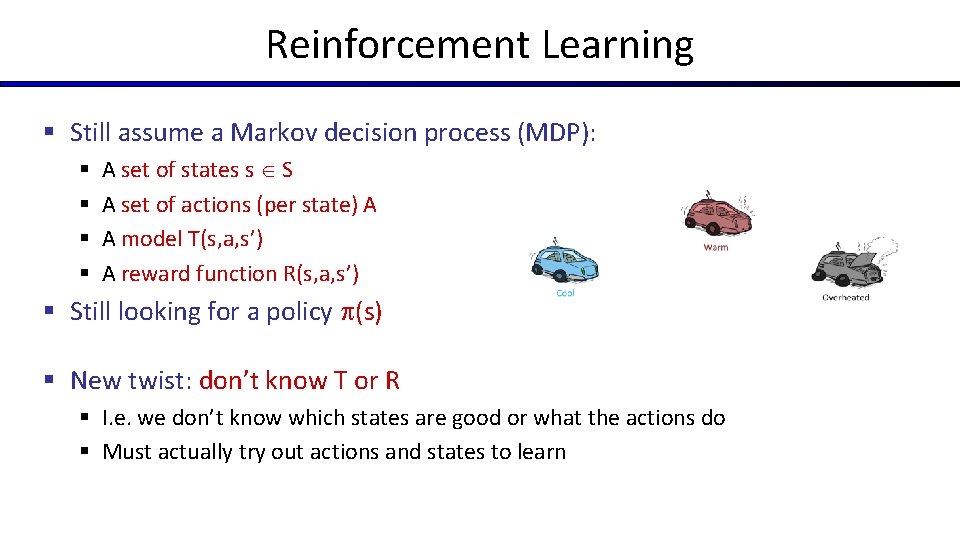
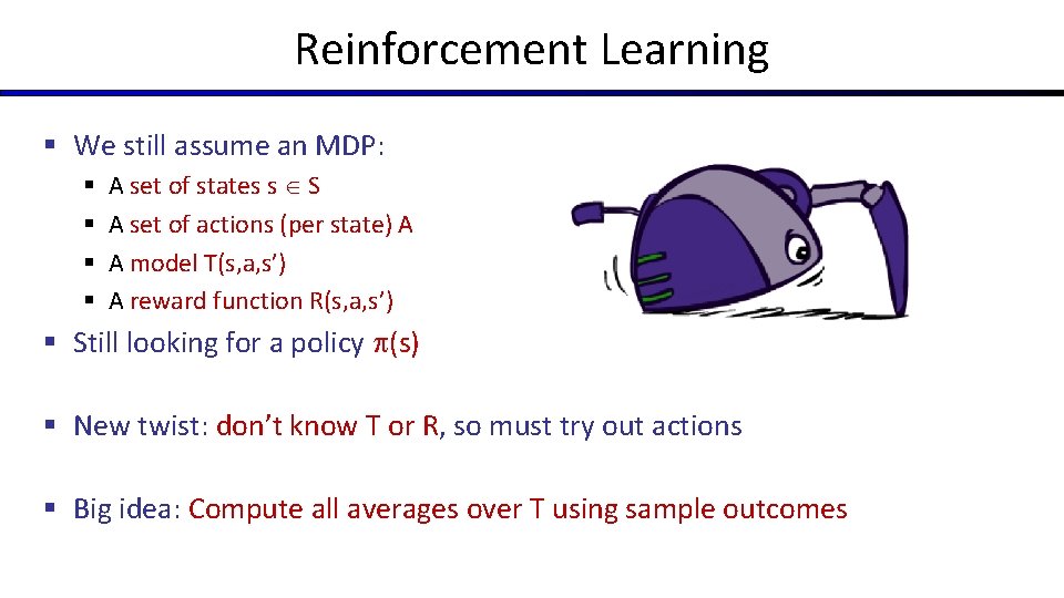
Reinforcement Learning § Still assume a Markov decision process (MDP): § § A set of states s S A set of actions (per state) A A model T(s, a, s’) A reward function R(s, a, s’) § Still looking for a policy (s) § New twist: don’t know T or R § I. e. we don’t know which states are good or what the actions do § Must actually try out actions and states to learn

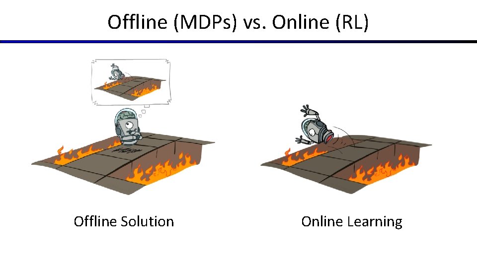
Offline (MDPs) vs. Online (RL) Offline Solution Online Learning

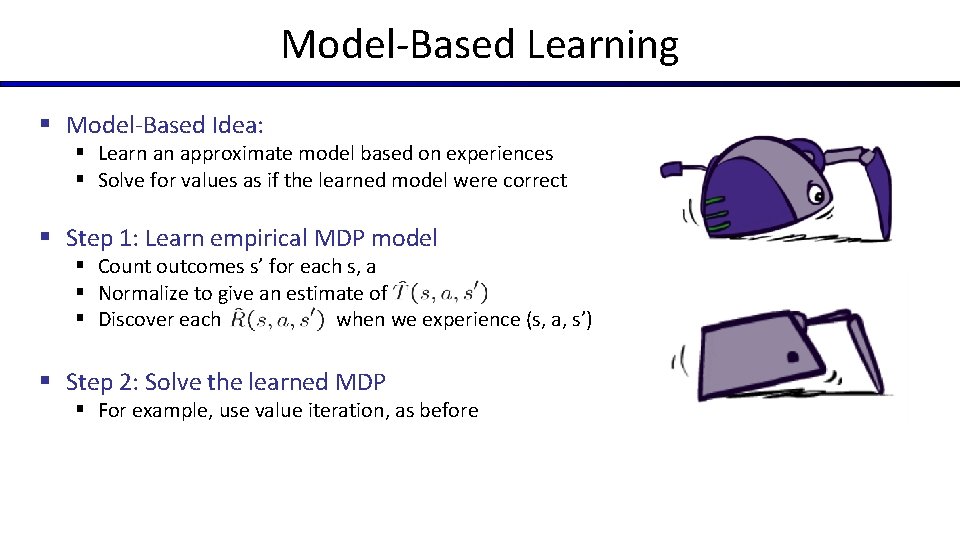
Model-Based Learning § Model-Based Idea: § Learn an approximate model based on experiences § Solve for values as if the learned model were correct § Step 1: Learn empirical MDP model § Count outcomes s’ for each s, a § Normalize to give an estimate of § Discover each when we experience (s, a, s’) § Step 2: Solve the learned MDP § For example, use value iteration, as before

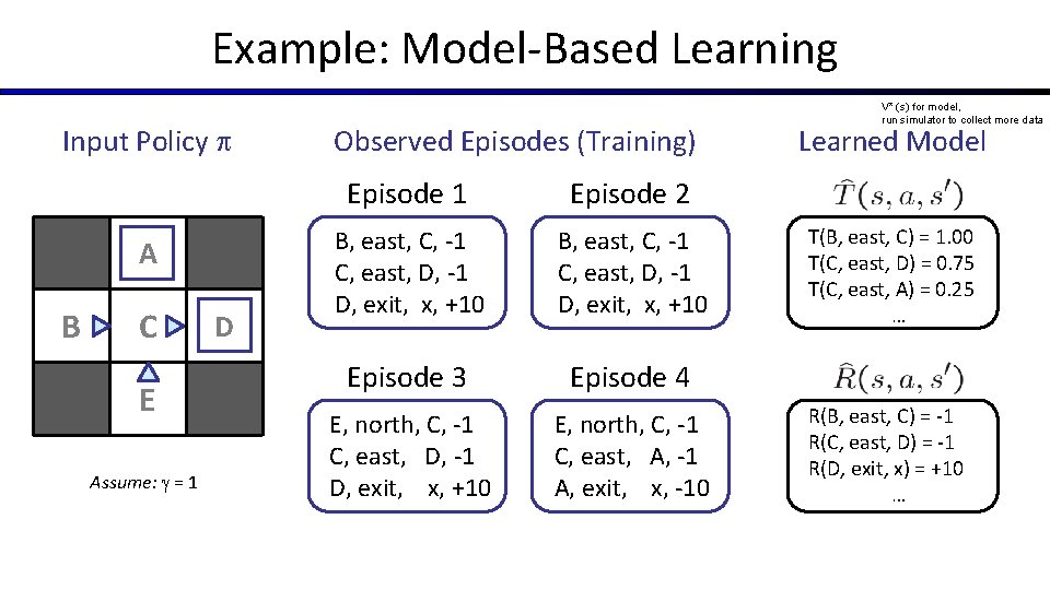
Example: Model-Based Learning Input Policy A B C E Assume: = 1 D Observed Episodes (Training) Episode 1 Episode 2 B, east, C, -1 C, east, D, -1 D, exit, x, +10 Episode 3 Episode 4 E, north, C, -1 C, east, D, -1 D, exit, x, +10 E, north, C, -1 C, east, A, -1 A, exit, x, -10 V* (s) for model, run simulator to collect more data Learned Model T(s, a, s’). T(B, east, C) = 1. 00 T(C, east, D) = 0. 75 T(C, east, A) = 0. 25 … R(s, a, s’). R(B, east, C) = -1 R(C, east, D) = -1 R(D, exit, x) = +10 …

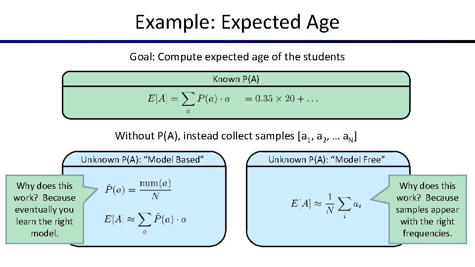
Example: Expected Age Goal: Compute expected age of the students Known P(A) Without P(A), instead collect samples [a 1, a 2, … a. N] Unknown P(A): “Model Based” Why does this work? Because eventually you learn the right model. Unknown P(A): “Model Free” Why does this work? Because samples appear with the right frequencies.

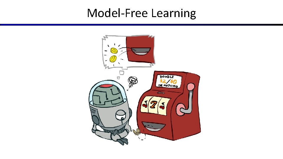
Model-Free Learning

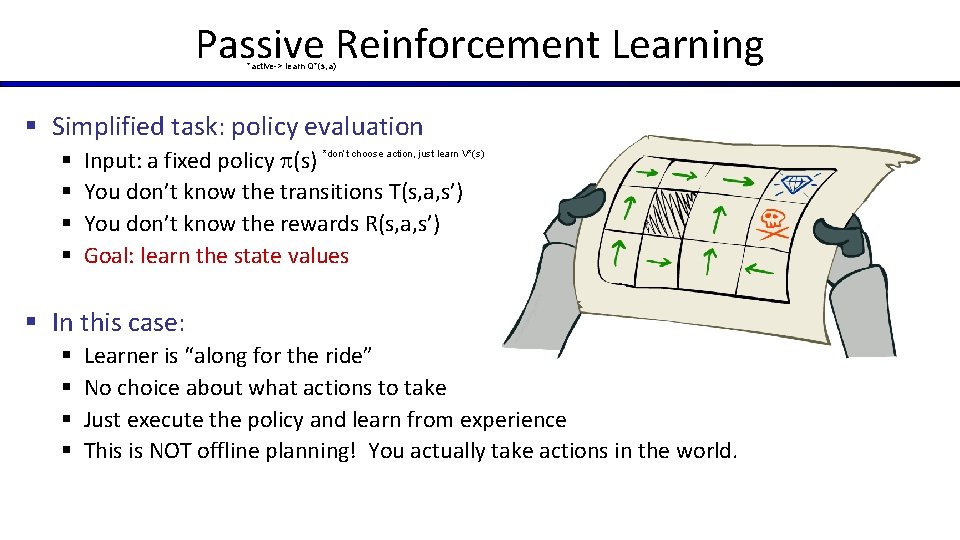
Passive Reinforcement Learning *active-> learn Q*(s, a) § Simplified task: policy evaluation § § Input: a fixed policy (s) *don’t choose action, just learn V*(s) You don’t know the transitions T(s, a, s’) You don’t know the rewards R(s, a, s’) Goal: learn the state values § In this case: § § Learner is “along for the ride” No choice about what actions to take Just execute the policy and learn from experience This is NOT offline planning! You actually take actions in the world.

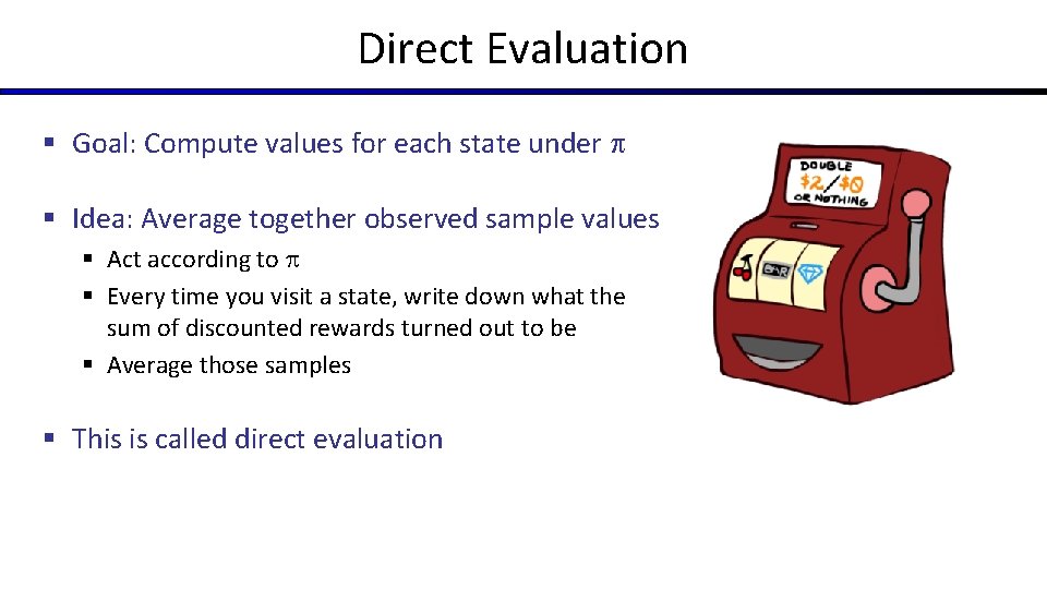
Direct Evaluation § Goal: Compute values for each state under § Idea: Average together observed sample values § Act according to § Every time you visit a state, write down what the sum of discounted rewards turned out to be § Average those samples § This is called direct evaluation

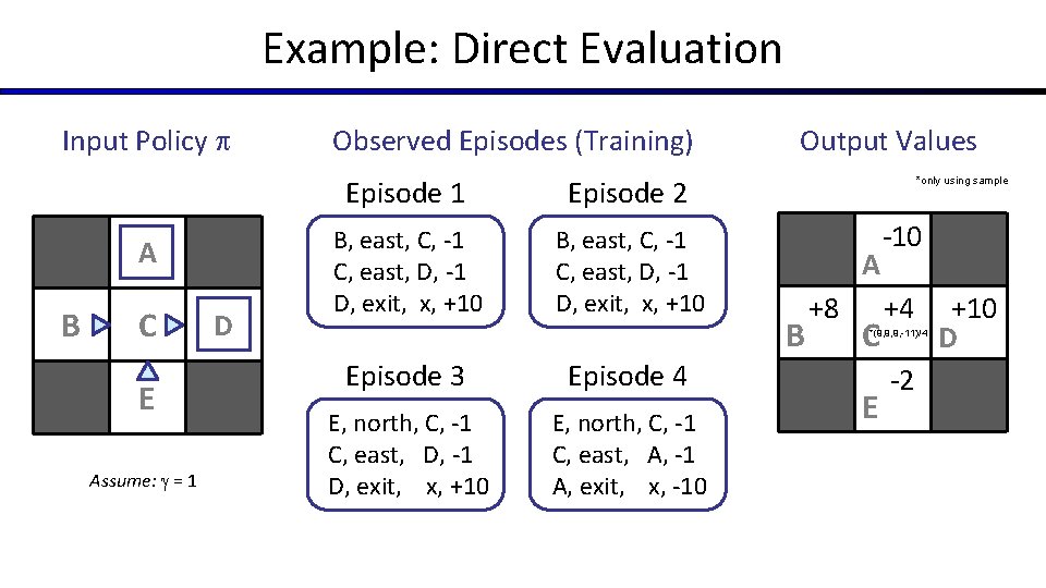
Example: Direct Evaluation Input Policy A B C E Assume: = 1 D Observed Episodes (Training) Episode 1 Episode 2 B, east, C, -1 C, east, D, -1 D, exit, x, +10 Episode 3 Episode 4 E, north, C, -1 C, east, D, -1 D, exit, x, +10 E, north, C, -1 C, east, A, -1 A, exit, x, -10 Output Values *only using sample A B +8 C -10 +4 *(9, 9, 9, -11)/4 E -2 +10 D

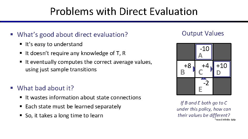
Problems with Direct Evaluation § What’s good about direct evaluation? § It’s easy to understand § It doesn’t require any knowledge of T, R § It eventually computes the correct average values, using just sample transitions § What bad about it? § It wastes information about state connections § Each state must be learned separately § So, it takes a long time to learn Output Values -10 A +8 +4 +10 B C D -2 E If B and E both go to C under this policy, how can their values be different? *need infinite data

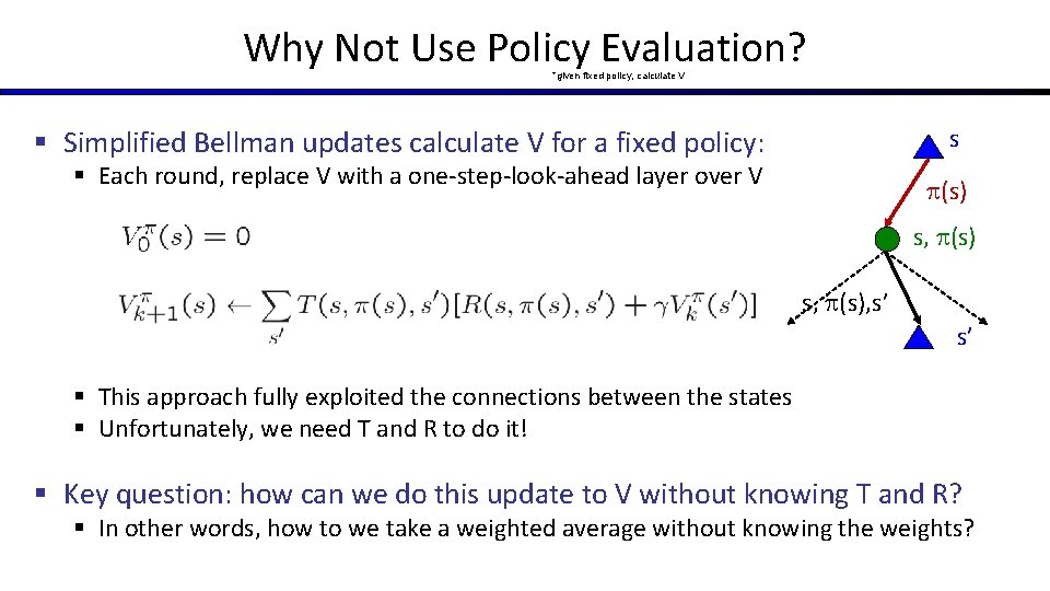
Why Not Use Policy Evaluation? *given fixed policy, calculate V s § Simplified Bellman updates calculate V for a fixed policy: § Each round, replace V with a one-step-look-ahead layer over V (s) s, (s), s’ s’ § This approach fully exploited the connections between the states § Unfortunately, we need T and R to do it! § Key question: how can we do this update to V without knowing T and R? § In other words, how to we take a weighted average without knowing the weights?

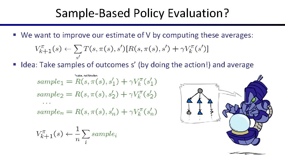
Sample-Based Policy Evaluation? § We want to improve our estimate of V by computing these averages: § Idea: Take samples of outcomes s’ (by doing the action!) and average *value, not function s (s) s, (s), s’ s 2' s 1' s' s 3' Almost! But we can’t rewind time to get sample after sample from state s.

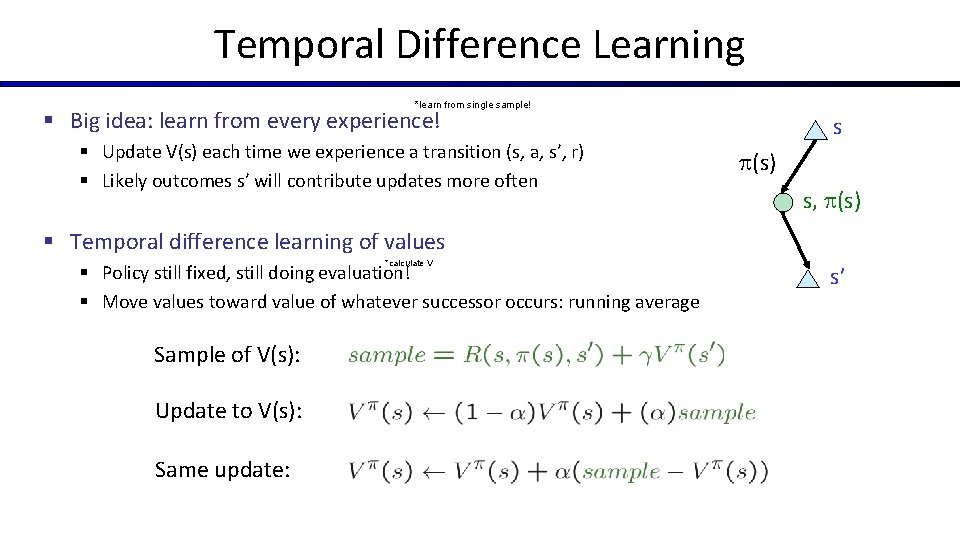
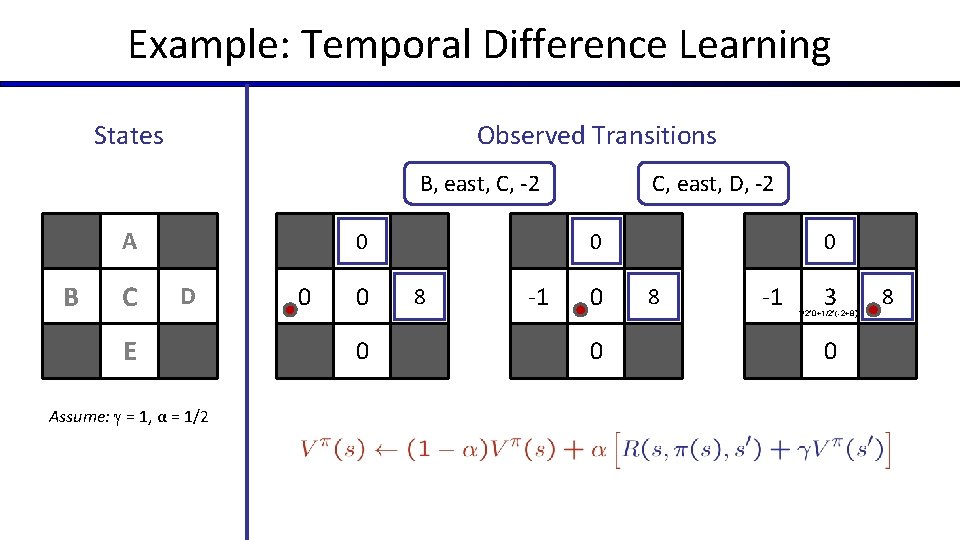
Temporal Difference Learning *learn from single sample! § Big idea: learn from every experience! § Update V(s) each time we experience a transition (s, a, s’, r) § Likely outcomes s’ will contribute updates more often s (s) s, (s) § Temporal difference learning of values *calculate V § Policy still fixed, still doing evaluation! § Move values toward value of whatever successor occurs: running average Sample of V(s): Update to V(s): Same update: s’

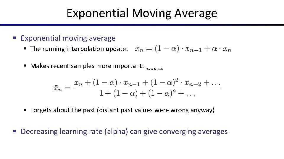
Exponential Moving Average § Exponential moving average § The running interpolation update: § Makes recent samples more important: *same formula § Forgets about the past (distant past values were wrong anyway) § Decreasing learning rate (alpha) can give converging averages

Example: Temporal Difference Learning States Observed Transitions B, east, C, -2 A B C 0 D E Assume: = 1, α = 1/2 0 0 0 C, east, D, -2 0 8 -1 0 0 0 8 -1 3 1/2*0+1/2*(-2+8 ) 0 8

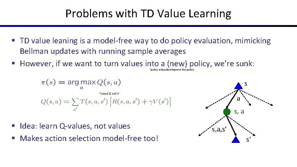
Problems with TD Value Learning § TD value leaning is a model-free way to do policy evaluation, mimicking Bellman updates with running sample averages § However, if we want to turn values into a (new) policy, we’re sunk: *policy extraction/improve the policy s *need Q not V a s, a § Idea: learn Q-values, not values § Makes action selection model-free too! s, a, s’ s’

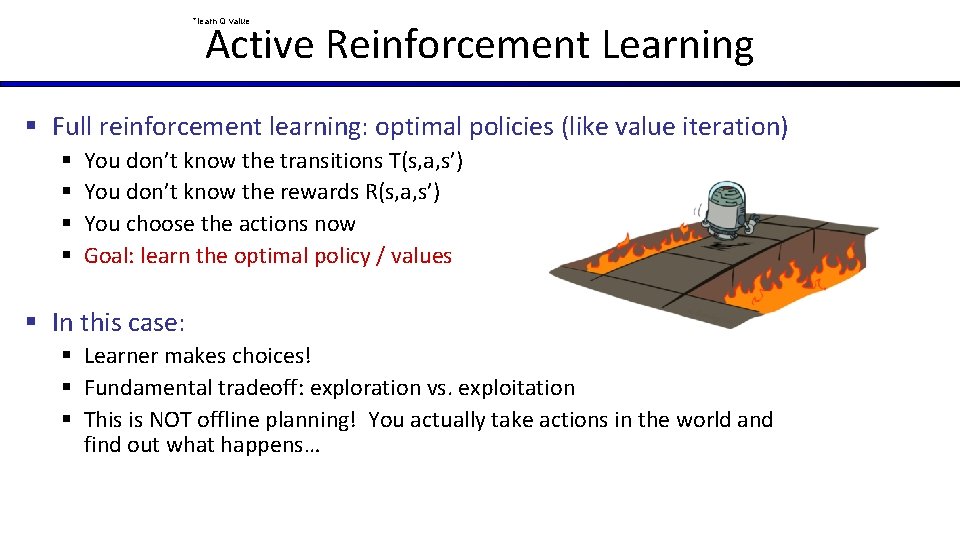
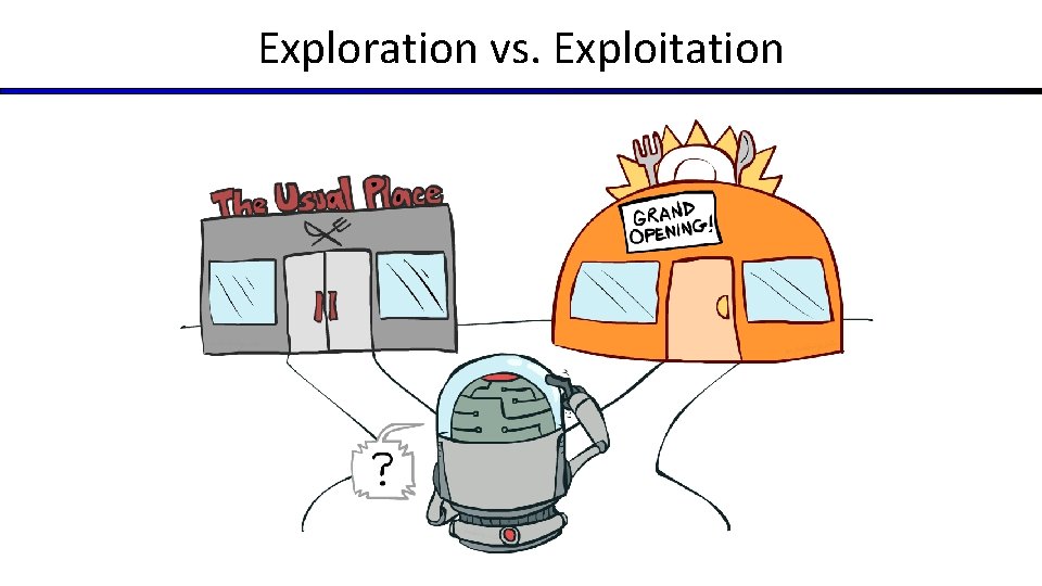
Active Reinforcement Learning *learn Q value § Full reinforcement learning: optimal policies (like value iteration) § § You don’t know the transitions T(s, a, s’) You don’t know the rewards R(s, a, s’) You choose the actions now Goal: learn the optimal policy / values § In this case: § Learner makes choices! § Fundamental tradeoff: exploration vs. exploitation § This is NOT offline planning! You actually take actions in the world and find out what happens…

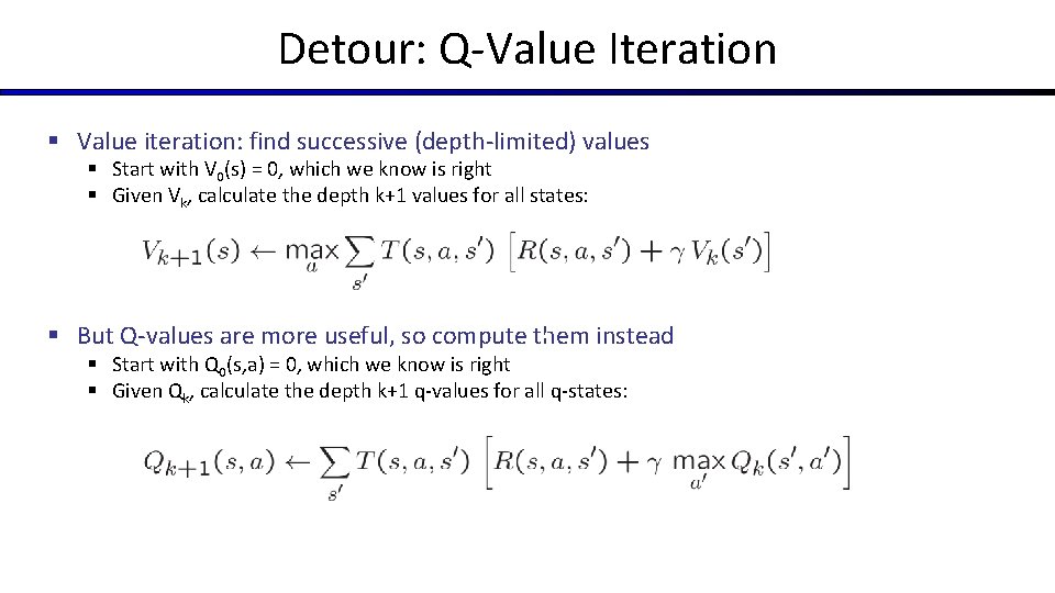
Detour: Q-Value Iteration § Value iteration: find successive (depth-limited) values § Start with V 0(s) = 0, which we know is right § Given Vk, calculate the depth k+1 values for all states: § But Q-values are more useful, so compute them instead § Start with Q 0(s, a) = 0, which we know is right § Given Qk, calculate the depth k+1 q-values for all q-states:

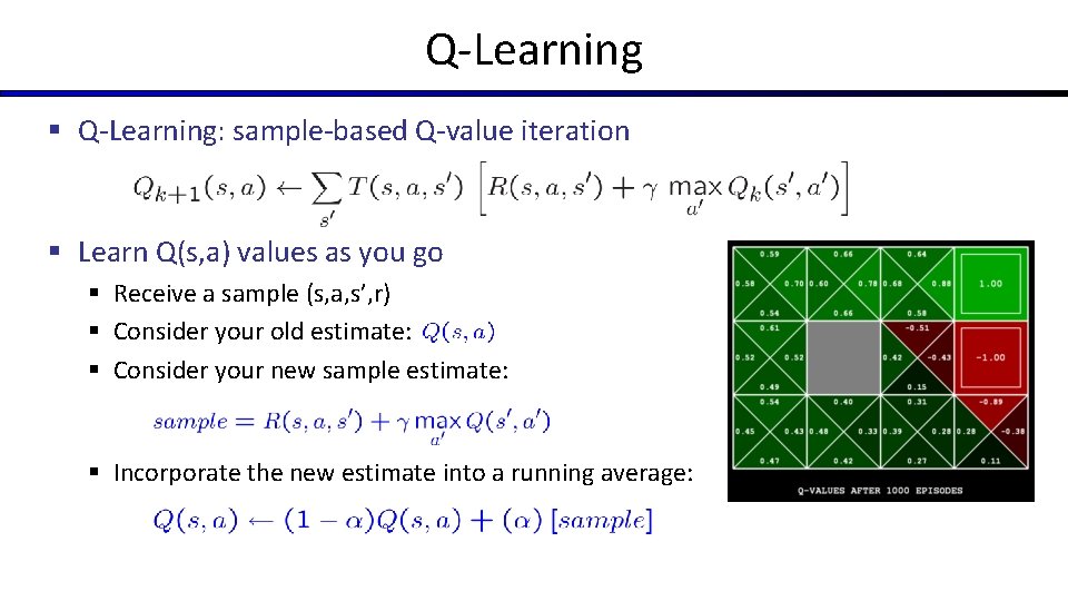
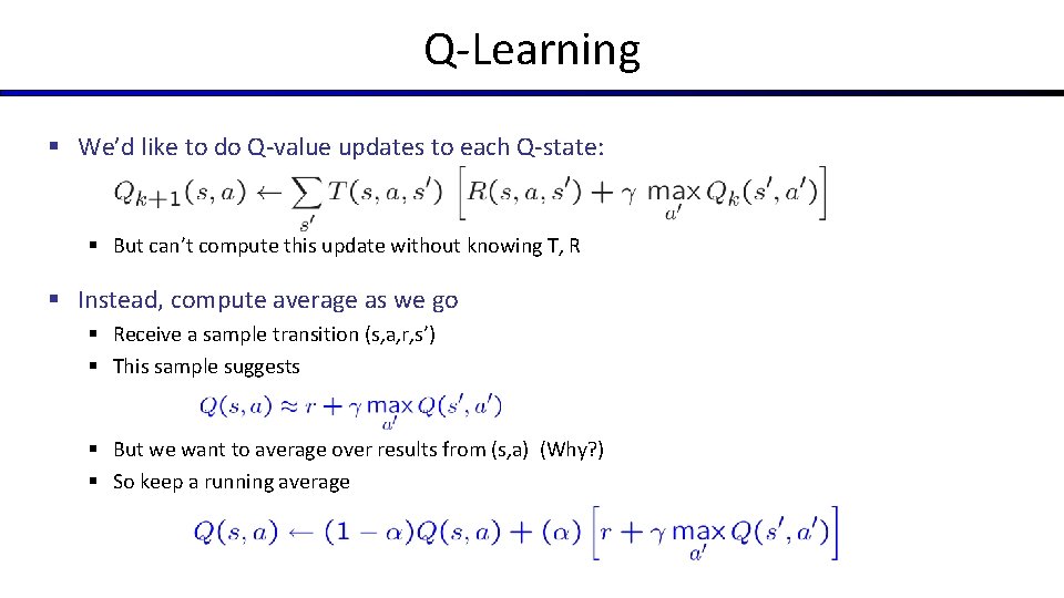
Q-Learning § Q-Learning: sample-based Q-value iteration § Learn Q(s, a) values as you go § Receive a sample (s, a, s’, r) § Consider your old estimate: § Consider your new sample estimate: § Incorporate the new estimate into a running average:

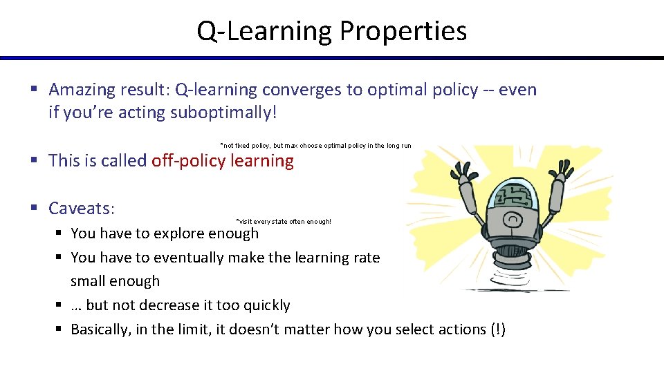
Q-Learning Properties § Amazing result: Q-learning converges to optimal policy -- even if you’re acting suboptimally! *not fixed policy, but max choose optimal policy in the long run § This is called off-policy learning § Caveats: *visit every state often enough! § You have to explore enough § You have to eventually make the learning rate small enough § … but not decrease it too quickly § Basically, in the limit, it doesn’t matter how you select actions (!)

Reinforcement Learning II

Reinforcement Learning § We still assume an MDP: § § A set of states s S A set of actions (per state) A A model T(s, a, s’) A reward function R(s, a, s’) § Still looking for a policy (s) § New twist: don’t know T or R, so must try out actions § Big idea: Compute all averages over T using sample outcomes

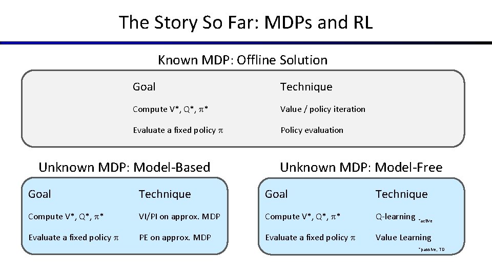
The Story So Far: MDPs and RL Known MDP: Offline Solution Goal Technique Compute V*, Q*, * Value / policy iteration Evaluate a fixed policy Policy evaluation Unknown MDP: Model-Based Unknown MDP: Model-Free Goal Technique Compute V*, Q*, * VI/PI on approx. MDP Compute V*, Q*, * Q-learning Evaluate a fixed policy PE on approx. MDP Evaluate a fixed policy Value Learning *active *passive, TD

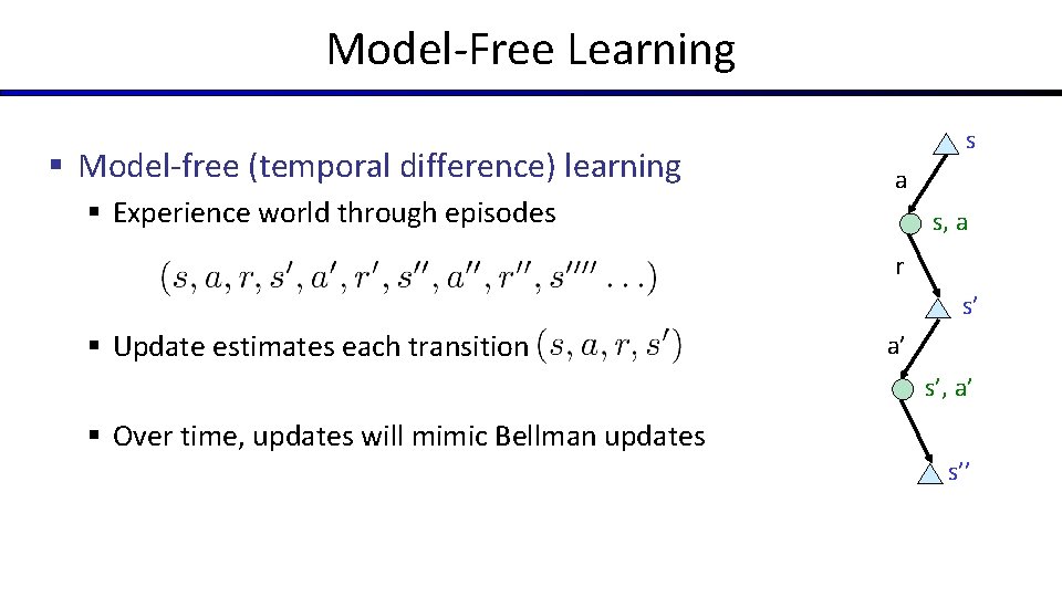
Model-Free Learning § Model-free (temporal difference) learning § Experience world through episodes s a s, a r s’ § Update estimates each transition a’ s’, a’ § Over time, updates will mimic Bellman updates s’’

Q-Learning § We’d like to do Q-value updates to each Q-state: § But can’t compute this update without knowing T, R § Instead, compute average as we go § Receive a sample transition (s, a, r, s’) § This sample suggests § But we want to average over results from (s, a) (Why? ) § So keep a running average

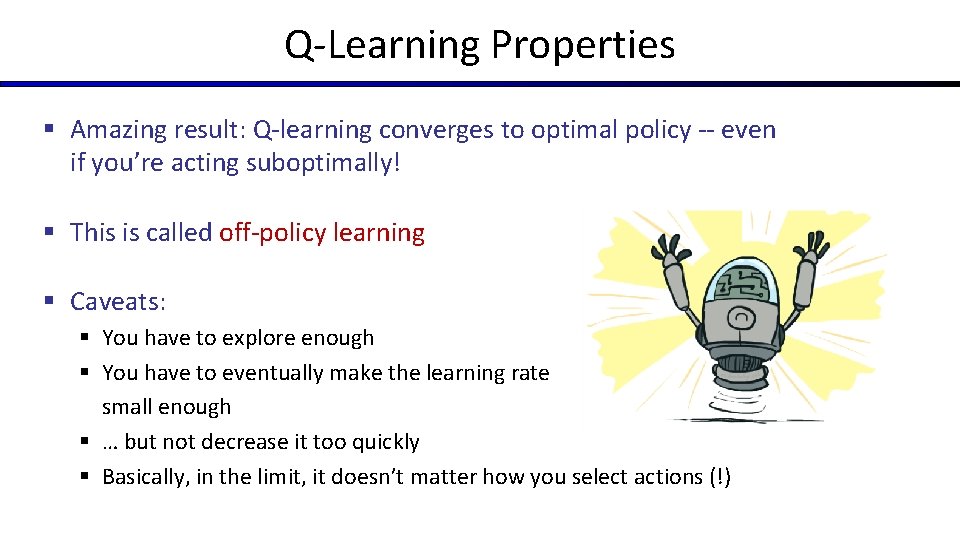
Q-Learning Properties § Amazing result: Q-learning converges to optimal policy -- even if you’re acting suboptimally! § This is called off-policy learning § Caveats: § You have to explore enough § You have to eventually make the learning rate small enough § … but not decrease it too quickly § Basically, in the limit, it doesn’t matter how you select actions (!)

Exploration vs. Exploitation

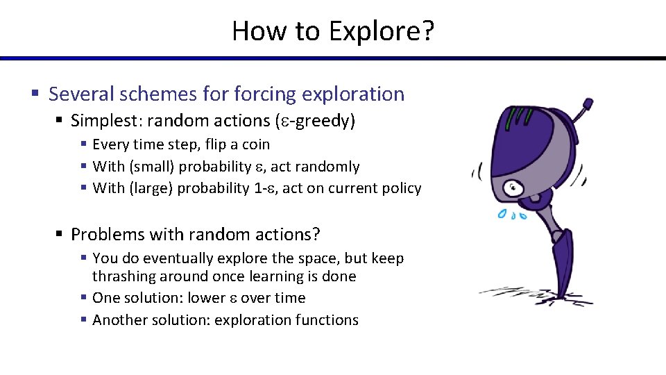
How to Explore? § Several schemes forcing exploration § Simplest: random actions ( -greedy) § Every time step, flip a coin § With (small) probability , act randomly § With (large) probability 1 - , act on current policy § Problems with random actions? § You do eventually explore the space, but keep thrashing around once learning is done § One solution: lower over time § Another solution: exploration functions

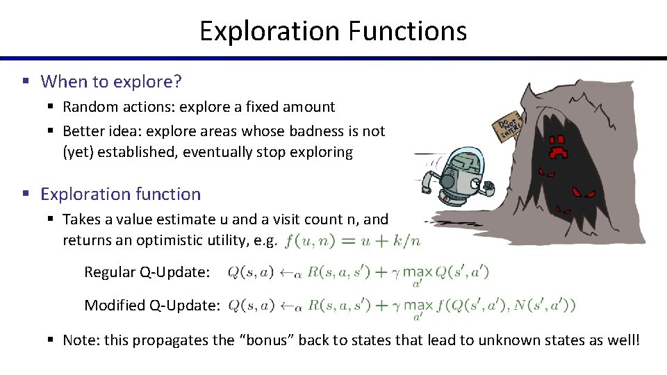
Exploration Functions § When to explore? § Random actions: explore a fixed amount § Better idea: explore areas whose badness is not (yet) established, eventually stop exploring § Exploration function § Takes a value estimate u and a visit count n, and returns an optimistic utility, e. g. Regular Q-Update: Modified Q-Update: § Note: this propagates the “bonus” back to states that lead to unknown states as well!

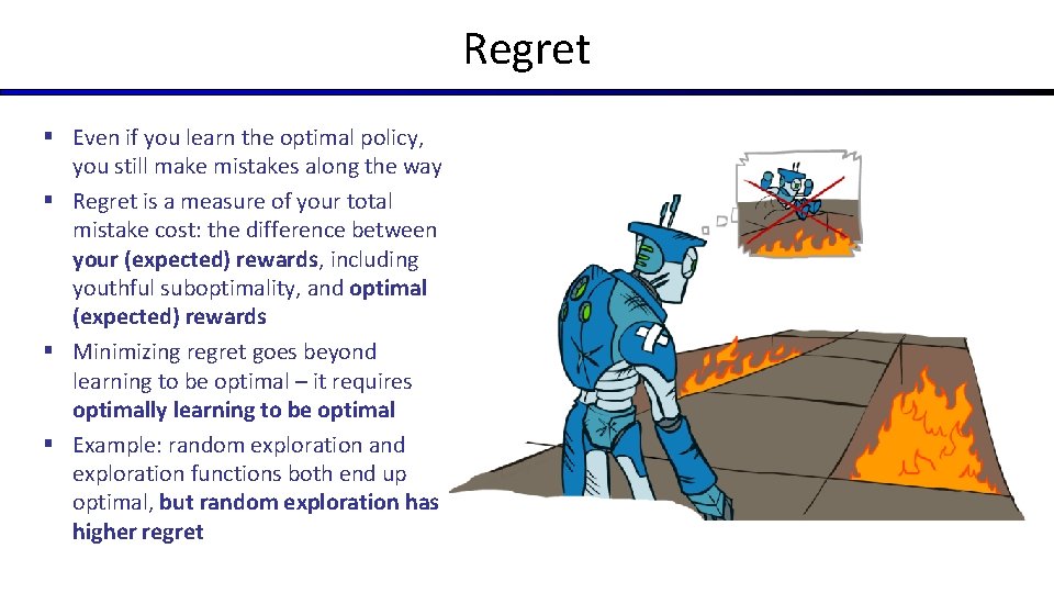
Regret § Even if you learn the optimal policy, you still make mistakes along the way! § Regret is a measure of your total mistake cost: the difference between your (expected) rewards, including youthful suboptimality, and optimal (expected) rewards § Minimizing regret goes beyond learning to be optimal – it requires optimally learning to be optimal § Example: random exploration and exploration functions both end up optimal, but random exploration has higher regret

Approximate Q-Learning

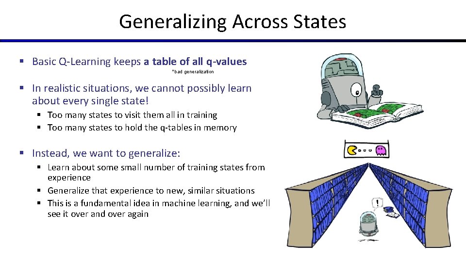
Generalizing Across States § Basic Q-Learning keeps a table of all q-values *bad generalization § In realistic situations, we cannot possibly learn about every single state! § Too many states to visit them all in training § Too many states to hold the q-tables in memory § Instead, we want to generalize: § Learn about some small number of training states from experience § Generalize that experience to new, similar situations § This is a fundamental idea in machine learning, and we’ll see it over and over again

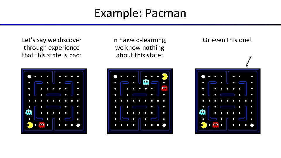
Example: Pacman Let’s say we discover through experience that this state is bad: In naïve q-learning, we know nothing about this state: Or even this one!

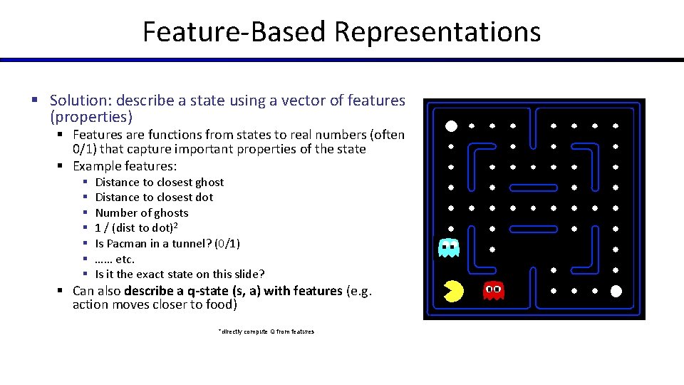
Feature-Based Representations § Solution: describe a state using a vector of features (properties) § Features are functions from states to real numbers (often 0/1) that capture important properties of the state § Example features: § § § § Distance to closest ghost Distance to closest dot Number of ghosts 1 / (dist to dot)2 Is Pacman in a tunnel? (0/1) …… etc. Is it the exact state on this slide? § Can also describe a q-state (s, a) with features (e. g. action moves closer to food) *directly compute Q from features

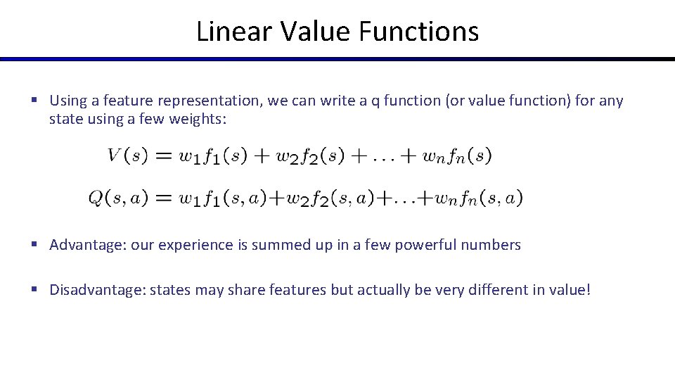
Linear Value Functions § Using a feature representation, we can write a q function (or value function) for any state using a few weights: § Advantage: our experience is summed up in a few powerful numbers § Disadvantage: states may share features but actually be very different in value!

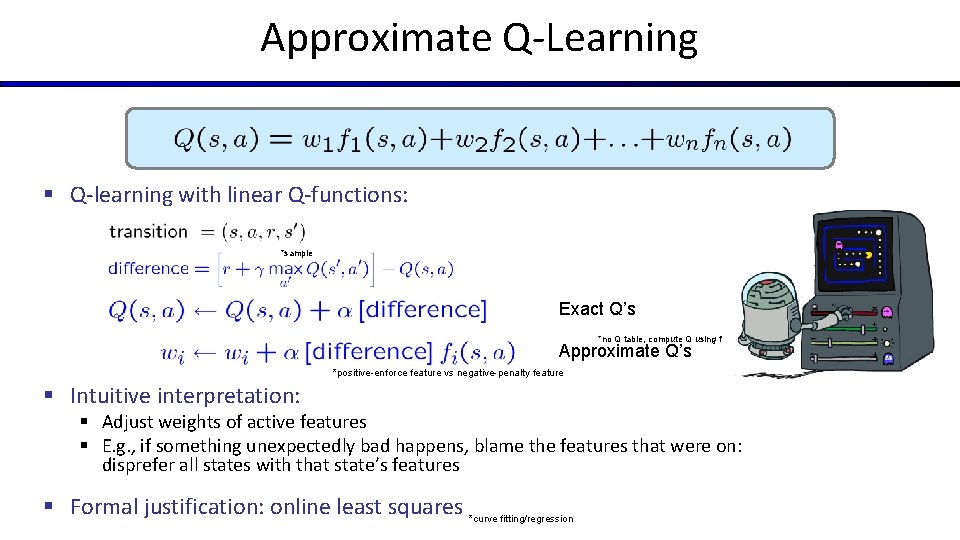
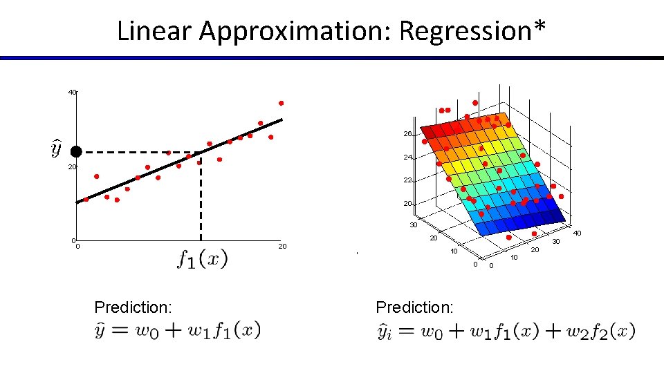
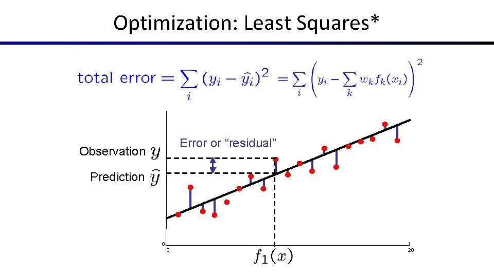
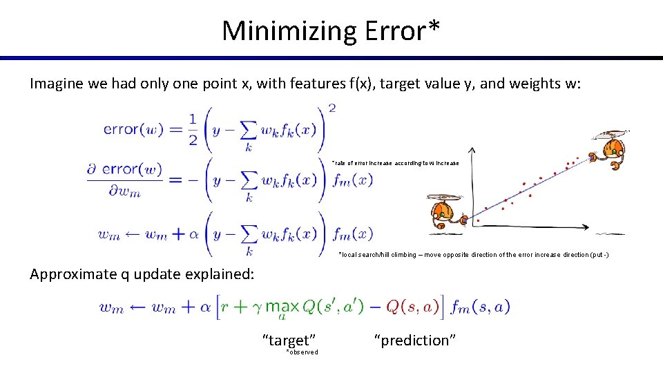
Approximate Q-Learning § Q-learning with linear Q-functions: *sample Exact Q’s *no Q table, compute Q using f Approximate Q’s *positive-enforce feature vs negative-penalty feature § Intuitive interpretation: § Adjust weights of active features § E. g. , if something unexpectedly bad happens, blame the features that were on: disprefer all states with that state’s features § Formal justification: online least squares *curve fitting/regression

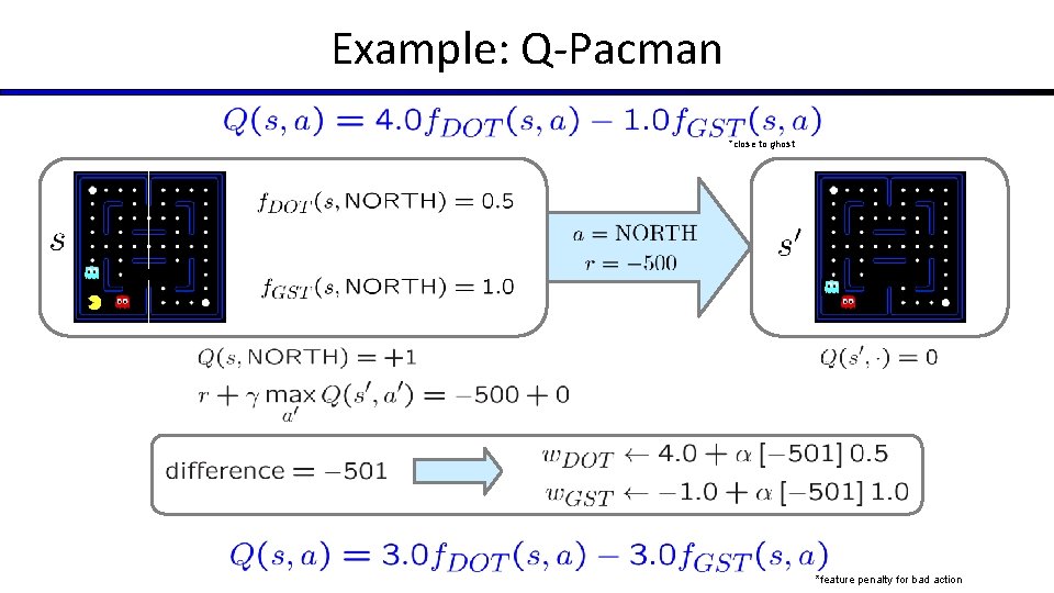
Example: Q-Pacman *close to ghost *feature penalty for bad action

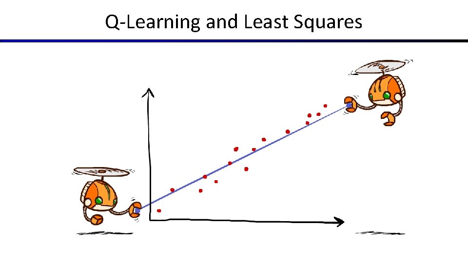
Q-Learning and Least Squares

Linear Approximation: Regression* 40 26 24 20 22 20 30 40 20 0 0 20 30 20 10 0 Prediction: 10 0

Optimization: Least Squares* Error or “residual” Observation Prediction 0 0 20

Minimizing Error* Imagine we had only one point x, with features f(x), target value y, and weights w: *rate of error increase according to w increase *local search/hill climbing – move opposite direction of the error increase direction (put -) Approximate q update explained: “target” *observed “prediction”

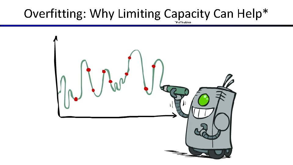
Overfitting: Why Limiting Capacity Can Help* *# of features 30 25 20 Degree 15 polynomial 15 10 5 0 -5 -10 -15 0 2 4 6 8 10 12 14 16 18 20

Policy Search *vs PI (Policy iteration)-Q learning § Problem: often the feature-based policies that work well (win games, maximize utilities) aren’t the ones that approximate V / Q best § E. g. your value functions were probably horrible estimates of future rewards, but they still produced good decisions § Q-learning’s priority: get Q-values close (modeling) *value != action (reward) § Action selection priority: get ordering of Q-values right (prediction) § We’ll see this distinction between modeling and prediction again later in the course *directly optimize action § Solution: learn policies that maximize rewards, not the values that predict them § Policy search: start with an ok solution (e. g. Q-learning) then fine-tune by hill climbing on feature weights

Policy Search § Simplest policy search: § Start with an initial linear value function or Q-function § Nudge each feature weight up and down and see if your policy is better than before § Problems: § How do we tell the policy got better? § Need to run many sample episodes! § If there a lot of features, this can be impractical § Better methods exploit lookahead structure, sample wisely, change multiple parameters… *interleave q-learning (policy iteration) with policy search –e. g. actor-critic method

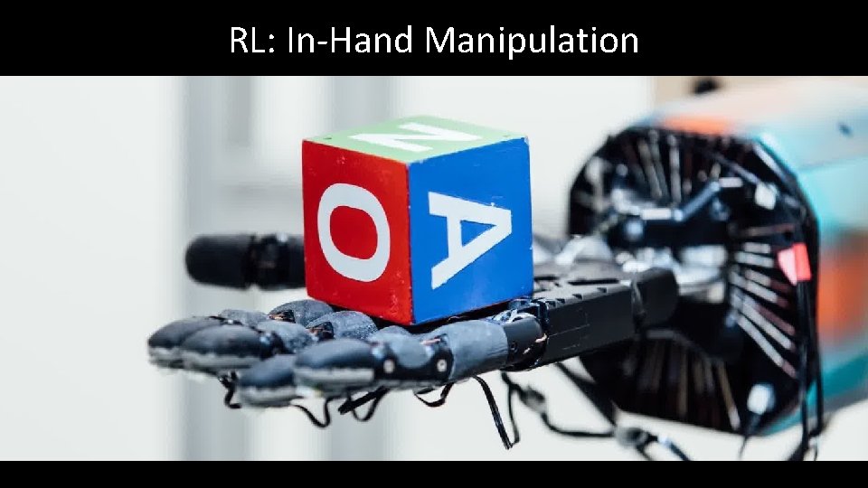
RL: In-Hand Manipulation Pieter Abbeel -- UC Berkeley | Gradescope | Covariant. AI