ECE517 Reinforcement Learning in Artificial Intelligence Lecture 10

ECE-517: Reinforcement Learning in Artificial Intelligence Lecture 10: Temporal-Difference Learning October 6, 2011 Dr. Itamar Arel College of Engineering Department of Electrical Engineering and Computer Science The University of Tennessee Fall 2011 1

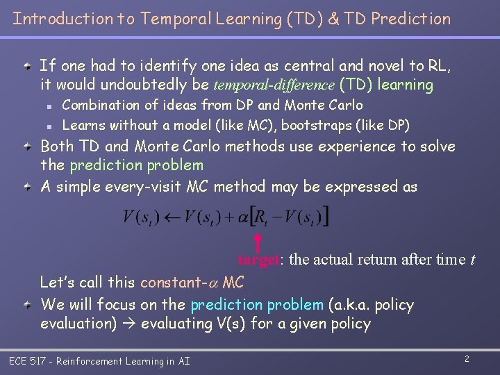
Introduction to Temporal Learning (TD) & TD Prediction If one had to identify one idea as central and novel to RL, it would undoubtedly be temporal-difference (TD) learning n n Combination of ideas from DP and Monte Carlo Learns without a model (like MC), bootstraps (like DP) Both TD and Monte Carlo methods use experience to solve the prediction problem A simple every-visit MC method may be expressed as target: the actual return after time t Let’s call this constant-a MC We will focus on the prediction problem (a. k. a. policy evaluation) evaluating V(s) for a given policy ECE 517 - Reinforcement Learning in AI 2

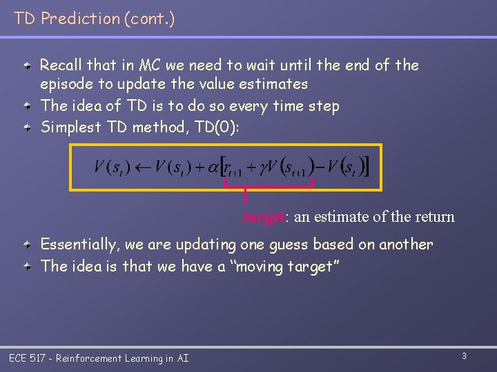
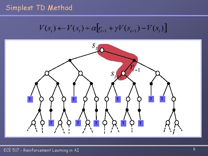
TD Prediction (cont. ) Recall that in MC we need to wait until the end of the episode to update the value estimates The idea of TD is to do so every time step Simplest TD method, TD(0): target: an estimate of the return Essentially, we are updating one guess based on another The idea is that we have a “moving target” ECE 517 - Reinforcement Learning in AI 3

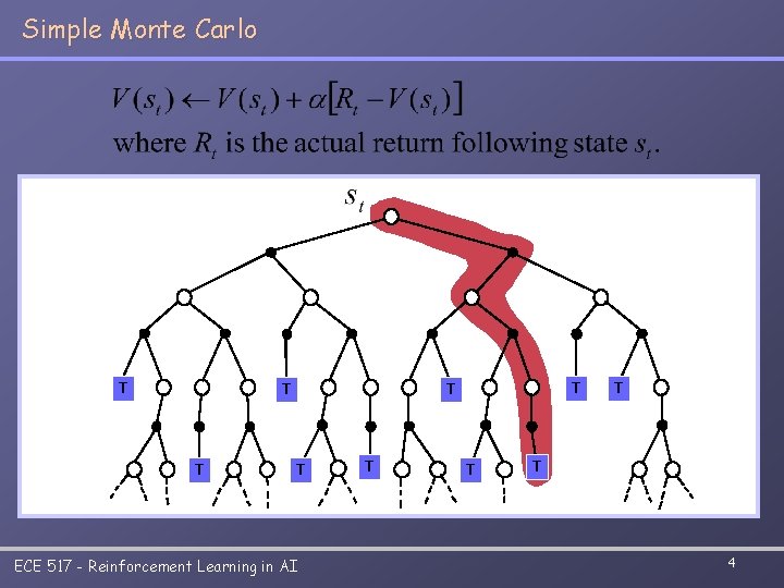
Simple Monte Carlo T TT T ECE 517 - Reinforcement Learning in AI TT T T TT 4

Simplest TD Method TT T T ECE 517 - Reinforcement Learning in AI TT T T TT 5

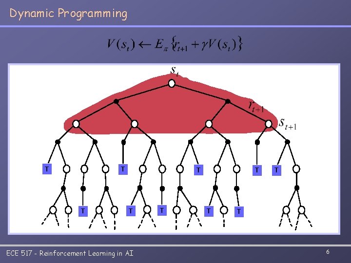
Dynamic Programming T TT TT T T ECE 517 - Reinforcement Learning in AI T T T 6

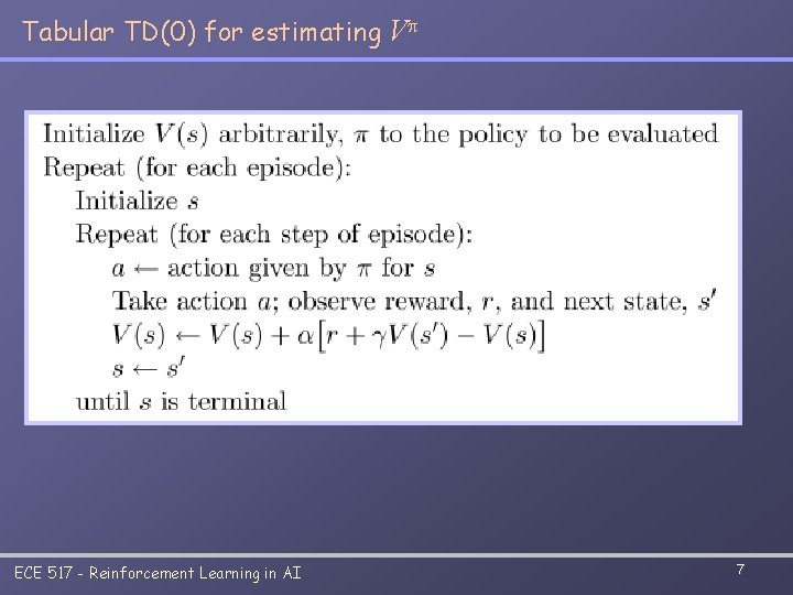
Tabular TD(0) for estimating Vp ECE 517 - Reinforcement Learning in AI 7

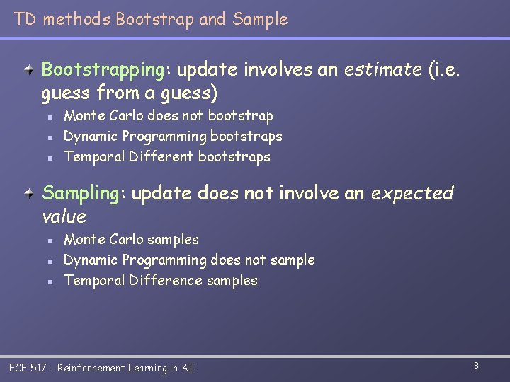
TD methods Bootstrap and Sample Bootstrapping: update involves an estimate (i. e. guess from a guess) n n n Monte Carlo does not bootstrap Dynamic Programming bootstraps Temporal Different bootstraps Sampling: update does not involve an expected value n n n Monte Carlo samples Dynamic Programming does not sample Temporal Difference samples ECE 517 - Reinforcement Learning in AI 8

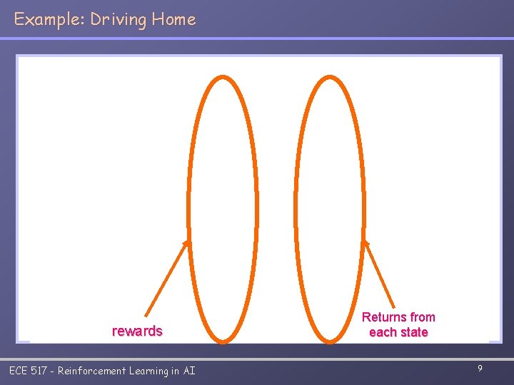
Example: Driving Home rewards ECE 517 - Reinforcement Learning in AI Returns from each state 9

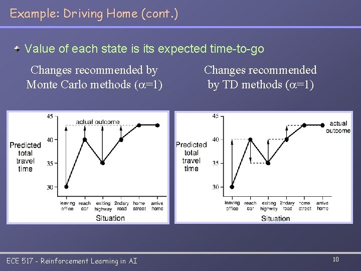
Example: Driving Home (cont. ) Value of each state is its expected time-to-go Changes recommended by Monte Carlo methods (a=1) ECE 517 - Reinforcement Learning in AI Changes recommended by TD methods (a=1) 10

Example: Driving Home (cont. ) Is it really necessary to wait until the end of the episode to start learning? n n Monte Carlo says it is TD learning argues that learning can occur on-line Suppose, on another day, you again estimate when leaving your office that it will take 30 minutes to drive home, but then you get stuck in a massive traffic jam n n n Twenty-five minutes after leaving the office you are still bumper-to-bumper on the highway You now estimate that it will take another 25 minutes to get home, for a total of 50 minutes Must you wait until you get home before increasing your estimate for the initial state? In TD you would be shifting your initial estimate from 30 minutes toward 50 ECE 517 - Reinforcement Learning in AI 11

Advantages of TD Learning TD methods do not require a model of the environment, only experience TD, but not MC, methods can be fully incremental n n Agent learns a “guess from a guess” Agent can learn before knowing the final outcome Less memory Reduced peak computation n Agent can learn without the final outcome From incomplete sequences Helps with applications that have very long episodes Both MC and TD converge (under certain assumptions to be detailed later), but which is faster? n Currently unknown – generally TD does better on stochastic tasks ECE 517 - Reinforcement Learning in AI 12

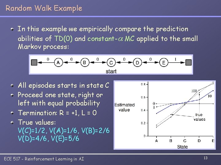
Random Walk Example In this example we empirically compare the prediction abilities of TD(0) and constant-a MC applied to the small Markov process: All episodes starts in state C Proceed one state, right or left with equal probability Termination: R = +1, L = 0 True values: V(C)=1/2, V(A)=1/6, V(B)=2/6 V(D)=4/6, V(E)=5/6 ECE 517 - Reinforcement Learning in AI 13

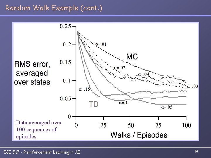
Random Walk Example (cont. ) Data averaged over 100 sequences of episodes ECE 517 - Reinforcement Learning in AI 14

Optimality of TD(0) Suppose only a finite amount of experience is available, say 10 episodes or 100 time steps Intuitively, we repeatedly present the experience until convergence is achieved Updates are made after a batch of training data n Also called batch updating For any finite Markov prediction task, under batch updating, TD(0) converges for sufficiently small a MC method also converges deterministically but to a different answer To better understand the different between MC and TD(0), we’ll consider the batch random walk ECE 517 - Reinforcement Learning in AI 15

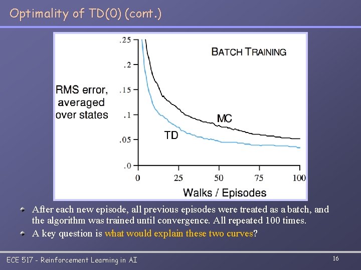
Optimality of TD(0) (cont. ) After each new episode, all previous episodes were treated as a batch, and the algorithm was trained until convergence. All repeated 100 times. A key question is what would explain these two curves? ECE 517 - Reinforcement Learning in AI 16

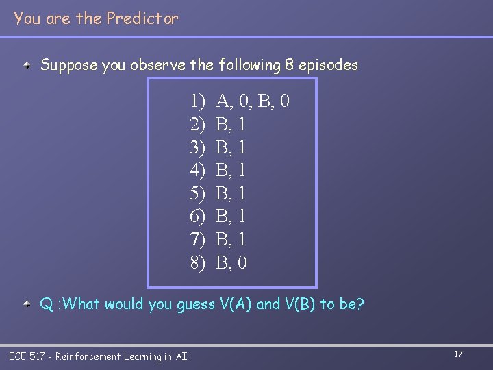
You are the Predictor Suppose you observe the following 8 episodes 1) 2) 3) 4) 5) 6) 7) 8) A, 0, B, 0 B, 1 B, 1 B, 0 Q : What would you guess V(A) and V(B) to be? ECE 517 - Reinforcement Learning in AI 17

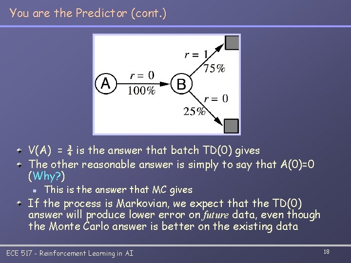
You are the Predictor (cont. ) V(A) = ¾ is the answer that batch TD(0) gives The other reasonable answer is simply to say that A(0)=0 (Why? ) n This is the answer that MC gives If the process is Markovian, we expect that the TD(0) answer will produce lower error on future data, even though the Monte Carlo answer is better on the existing data ECE 517 - Reinforcement Learning in AI 18

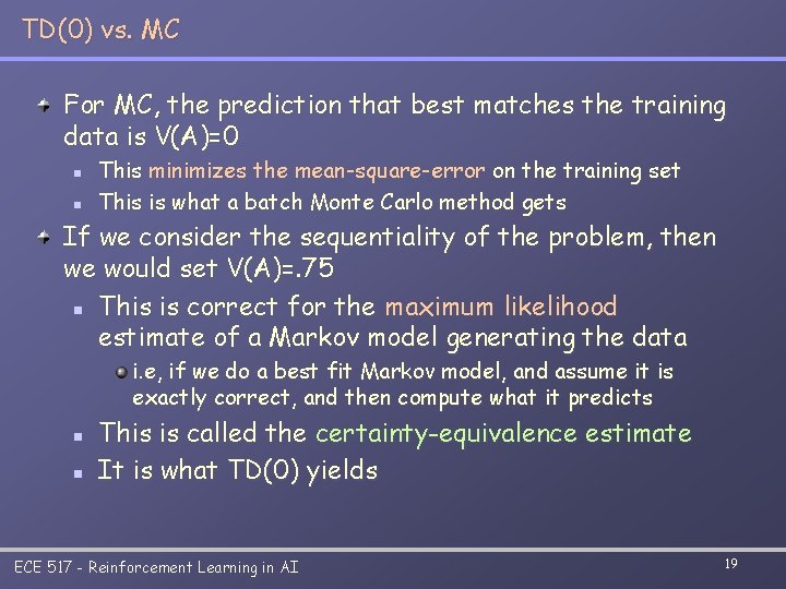
TD(0) vs. MC For MC, the prediction that best matches the training data is V(A)=0 n n This minimizes the mean-square-error on the training set This is what a batch Monte Carlo method gets If we consider the sequentiality of the problem, then we would set V(A)=. 75 n This is correct for the maximum likelihood estimate of a Markov model generating the data i. e, if we do a best fit Markov model, and assume it is exactly correct, and then compute what it predicts n n This is called the certainty-equivalence estimate It is what TD(0) yields ECE 517 - Reinforcement Learning in AI 19

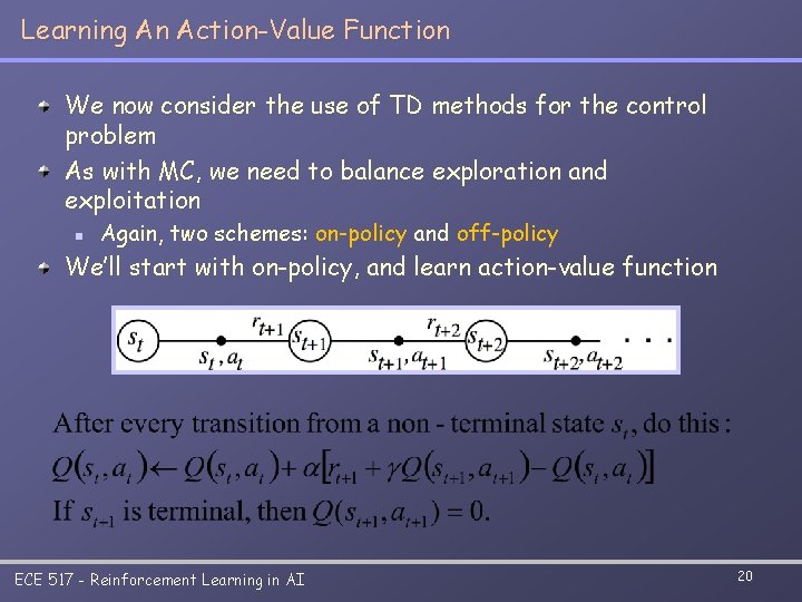
Learning An Action-Value Function We now consider the use of TD methods for the control problem As with MC, we need to balance exploration and exploitation n Again, two schemes: on-policy and off-policy We’ll start with on-policy, and learn action-value function ECE 517 - Reinforcement Learning in AI 20

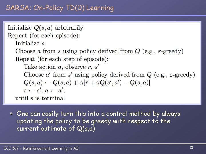
SARSA: On-Policy TD(0) Learning One can easily turn this into a control method by always updating the policy to be greedy with respect to the current estimate of Q(s, a) ECE 517 - Reinforcement Learning in AI 21

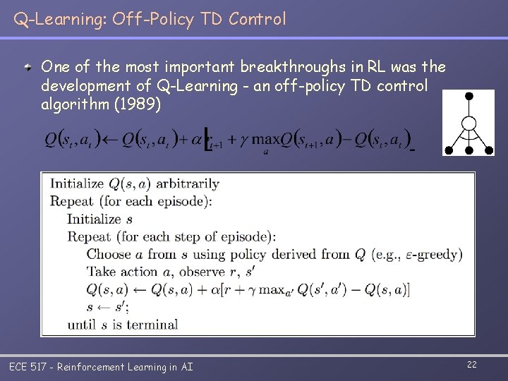
Q-Learning: Off-Policy TD Control One of the most important breakthroughs in RL was the development of Q-Learning - an off-policy TD control algorithm (1989) ECE 517 - Reinforcement Learning in AI 22

Q-Learning: Off-Policy TD Control (cont. ) The learned action-value function, Q, directly approximates the optimal action-value function, Q* Converges as long as all states are visited and state-action values updated Why is it considered an off-policy control method? How expensive is it to implement? ECE 517 - Reinforcement Learning in AI 23