Search Problems CSD 15 780 Graduate Artificial Intelligence

Search Problems CSD 15 -780: Graduate Artificial Intelligence Instructors: Zico Kolter and Zack Rubinstein TA: Vittorio Perera 1

Search n n Search lectures. Readings: n Section II in Norvig and Russel (chapters 3, 4, 5, and 6) 2

Today’s lecture n n n Why is search the key problem-solving technique in AI? Formulating and solving search problems. Understanding and comparing several “blind” or uniformed search techniques. 3

Projects Multi-robot movement planner for robust, just -in-time delivery of components for wing ladder assembly (Boeing) Assessment Region REVAMP - Same-day scheduler and real-time itinerary execution management support for paratransit operations. (ongoing ACCESS pilot) MARTI – Market-based dynamic allocation of tasks to RF devices to perform secondary mission requests (DARPA Radio. Map) SURTRAC - Adaptive traffic signalization control system • Focus on evaluation (pilot and expansion) SMOS - Cross-operations (air, cyber, space) coarselevel planner for missions (BAE and AFRL) ICLL

Examples of “toy” problems n Puzzles such as the 8 -puzzle: n Cryptarithmetic problems: SEND MORE MONEY 9567 +1085 10652 5

The n-queens problem n n A popular benchmark for AI search Solved for n up to 500, 000 6

Explicit solution for n ≥ 4 [Hoffman, Loessi, and Moore, 1969] If n is even but not of the form 6 k+2: For j = 1, 2, . . . , n/2 place queens on elements (j, 2 j), (n/2+j, 2 j-1) If n is even but not of the form 6 k: For j = 1, 2, . . . , n/2 place queens on elements (j, 1+[(2(j-1) + n/2 - 1) mod n]), (n+1 -j, n-[(2(j-1) + n/2 - 1) mod n]) If n is odd: Use case A or B on n-1 and extend with a queen at (n, n) Is this a good benchmark problem for testing search techniques? 7

Real-world problems n n n Signal interpretation (e. g. speech understanding) Theorem proving (e. g. resolution techniques) Combinatorial optimization (e. g. VLSI layout) Robot navigation (e. g. path planning) Factory scheduling (e. g. flexible manufacturing) Symbolic computation (e. g. symbolic integration) Can we find closed form solutions to these problems? 8

Formulating search problems n n n States and state spaces Operators - representing possible actions Successor function Initial state and goal test Path cost function Examples: 8 -puzzle, 8 -queen, path planning, map coloring. What are the corresponding states, operators, initial state, goal test, and path cost. 9

States, Operators, Successor function. State – choose data representation, e. g. , 3 x 3 2 D array with numbers and 0 representing the blank. move-left, move-right, move-up, move-down. Operators – transform state to next state, e. g. , possible movements for the blank. Successor Function – generate possible states by applying operators, e. g. , apply operators and return states whose indices are between 1 and 3. 10

What is a solution? n n n A solution to a search problem is a sequence of operators that generate a path from the initial state to a goal state. An optimal solution is a minimal cost solution. Solution cost versus search cost. 11

Choosing states and actions n n Efficiency versus expressiveness The use of abstraction: n n Ignore road condition travel planning. Use job description and ignore names in task scheduling. Ignore the color of the pieces when solving the 8 -puzzle. Compact action representation. 12

Quote for the day “The problem of searching a graph has effectively been solved, and is no longer of interest to AI researchers. ” - Nilsson, early 1970 s 13

Searching for solutions Search control strategies n Order in which the search space is explored n The extent to which partial solutions are kept and used to guide the search process n The degree to which the search process is guided by domain knowledge n The degree to which control decisions are made dynamically at run-time 14

Evaluation of search strategies n n Completeness - does it guarantee to find a solution when there is one? Time complexity - how long does it take to find a solution? Space complexity - how much memory does it require? Optimality - does it return the best solution when there are many? 15

Search trees n n n A graph representing the search process Implicit graphs and explicit graphs Branching factor and depth Generating and expanding states Open and closed lists of nodes Representing a node of the explicit graph: class Node: State = None Parent. Node = None Operator = None Depth = None Path. Cost = None 16

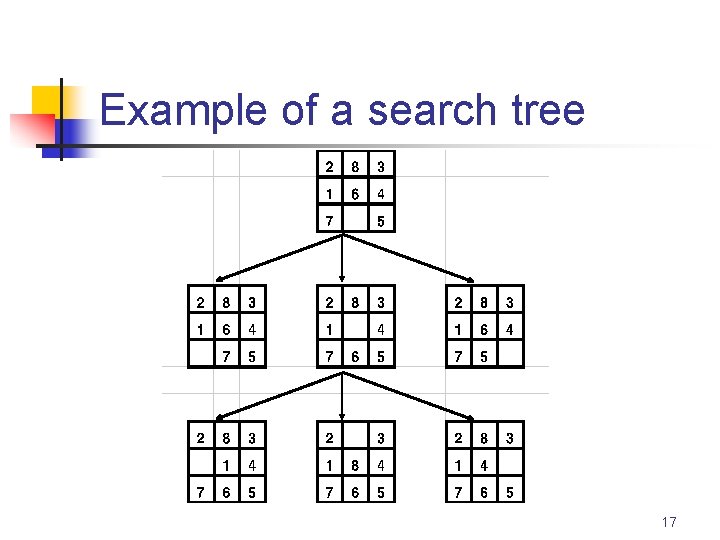
Example of a search tree 17

Blind search strategies n n n Depth-first search Breadth-first search Depth-limited search Iterative-deepening search Bidirectional search 18

Depth-First Search function dfs (nodes, goalp, successors) returns solution or fail if not nodes then return fail else if goalp(first(nodes)) then return first(nodes) else return dfs(append(successors(first(nodes)), rest(nodes)), goalp, successors) 19

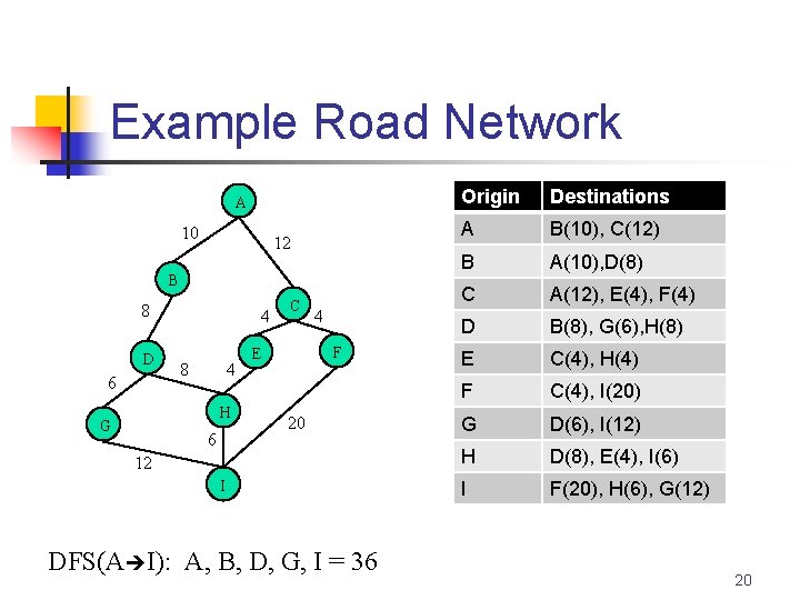
Example Road Network A 10 12 B 8 D 6 4 8 4 H G 6 C 4 F E 20 12 I DFS(A I): A, B, D, G, I = 36 Origin Destinations A B(10), C(12) B A(10), D(8) C A(12), E(4), F(4) D B(8), G(6), H(8) E C(4), H(4) F C(4), I(20) G D(6), I(12) H D(8), E(4), I(6) I F(20), H(6), G(12) 20

Time and Space Complexity of DFS n n n Let b be the branching factor and m be the maximum depth of the state space. Space complexity = bm Time complexity = O(bm) Complete? Optimal? 21

Breadth-First Search function bfs (nodes, goalp, successors) returns solution or fail if not nodes then return fail else if goalp(first(nodes)) then return first(nodes) else return dfs(append(rest(nodes), successors(first(nodes))), goalp, successors) 22

Example Road Network A 10 12 B 8 D 6 4 8 4 H G 6 C 4 F E 20 12 I BFS(A I): A, C, F, I = 36 Origin Destinations A B(10), C(12) B A(10), D(8) C A(12), E(4), F(4) D B(8), G(6), H(8) E C(4), H(4) F C(4), I(20) G D(6), I(12) H D(8), E(4), I(6) I F(20), H(6), G(12) 23

Time and Space Complexity of BFS n n n Let b be the branching factor and d be the depth at which a solution is found. Space complexity = O(bd) Time complexity = O(bd) Complete? Optimal? 24

Uniform-Cost Search function ucs (nodes, goalp, successors) returns solution or fail nodes = sort(<, nodes, node. cost) if not nodes then return fail else if goalp(first(nodes)) then return first(nodes) else return ucs(append(rest(nodes), successors(first(nodes))), goalp, successors) n Time and space complexity? 25

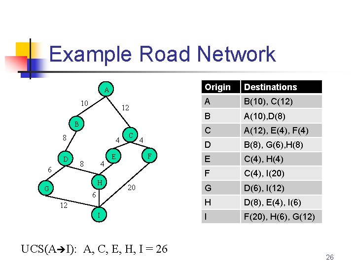
Example Road Network A 10 12 B 8 D 6 4 8 4 H G 6 C 4 F E 20 12 I UCS(A I): A, C, E, H, I = 26 Origin Destinations A B(10), C(12) B A(10), D(8) C A(12), E(4), F(4) D B(8), G(6), H(8) E C(4), H(4) F C(4), I(20) G D(6), I(12) H D(8), E(4), I(6) I F(20), H(6), G(12) 26

Uniform Cost Search Properties n n Guaranteed to find lowest cost solution (optimal and complete) as long as cost never decreases. Same complexity as Breadth-First search n n Space complexity = O(bd) Time complexity = O(bd) 27

Depth-Limited Search n n n Same as DFS, except depth threshold used to limit search. Similar time and space complexity to DFS, except bounded by threshold. Be careful to choose an appropriate threshold n n Complete? Optimal? 28

Example Road Network A 10 12 B 8 D 6 4 8 4 H G 6 C 4 F E 20 12 I DLS(A I, 4): A, B, D, G, I = 36 Origin Destinations A B(10), C(12) B A(10), D(8) C A(12), E(4), F(4) D B(8), G(6), H(8) E C(4), H(4) F C(4), I(20) G D(6), I(12) H D(8), E(4), I(6) I F(20), H(6), G(12) 29

Iterative Deepening Search n n Do repeated Depth-Limited searches, while incrementally increasing the threshold. Similar time and space complexity to DFS, except bounded by depth of the solution. n n Does redundant expansions. Is complete and optimal. 30

Example Road Network A 10 12 B 8 D 6 4 8 4 H G 6 C 4 F E 20 12 I IDS(A I): A, C, F, I = 36 Origin Destinations A B(10), C(12) B A(10), D(8) C A(12), E(4), F(4) D B(8), G(6), H(8) E C(4), H(4) F C(4), I(20) G D(6), I(12) H D(8), E(4), I(6) I F(20), H(6), G(12) 31

Bidirectional search n Time and space complexity: bd/2 When is bidirectional search applicable? 32

Time and Space Complexity of Bidirectional Search n n Time Complexity = O(bd/2) Space Complexity = O(bd/2) n High space complexity because the nodes have to be kept in memory to test for intersection of the two frontiers. 33

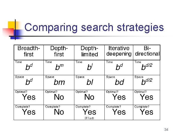
Comparing search strategies 34