Data Mining Cluster Analysis Advanced Concepts and Algorithms

Data Mining Cluster Analysis: Advanced Concepts and Algorithms Lecture Notes for Chapter 9 Introduction to Data Mining by Tan, Steinbach, Kumar © Tan, Steinbach, Kumar Introduction to Data Mining 4/18/2004 1

Hierarchical Clustering: Revisited l Creates nested clusters l Agglomerative clustering algorithms vary in terms of how the proximity of two clusters are computed u MIN (single link): susceptible to noise/outliers u MAX/GROUP AVERAGE: may not work well with non-globular clusters – CURE algorithm tries to handle both problems l Often starts with a proximity matrix – A type of graph-based algorithm © Tan, Steinbach, Kumar Introduction to Data Mining 4/18/2004 2

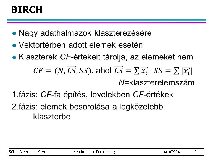
BIRCH l © Tan, Steinbach, Kumar Introduction to Data Mining 4/18/2004 3

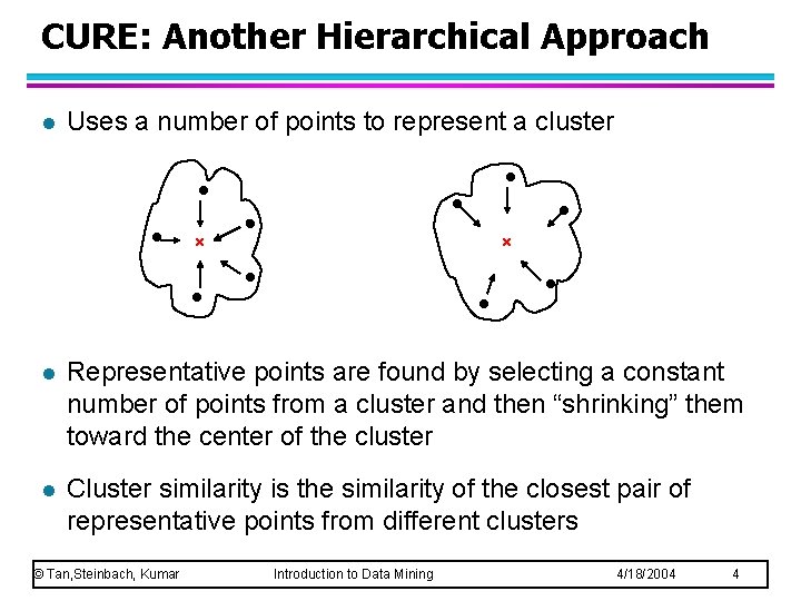
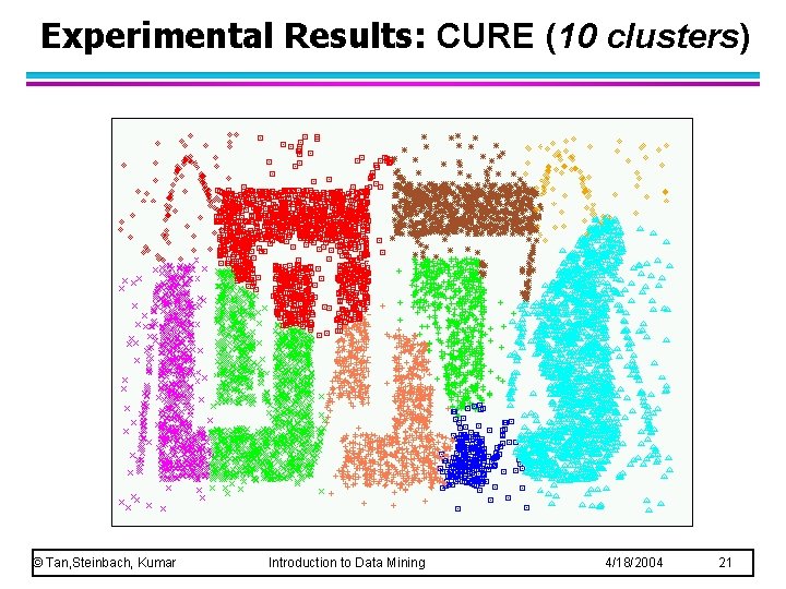
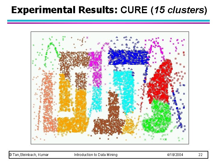
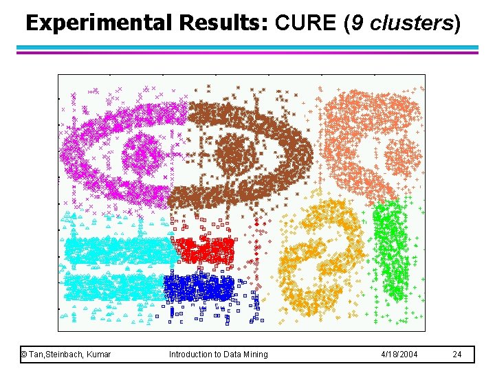
CURE: Another Hierarchical Approach l Uses a number of points to represent a cluster l Representative points are found by selecting a constant number of points from a cluster and then “shrinking” them toward the center of the cluster l Cluster similarity is the similarity of the closest pair of representative points from different clusters © Tan, Steinbach, Kumar Introduction to Data Mining 4/18/2004 4

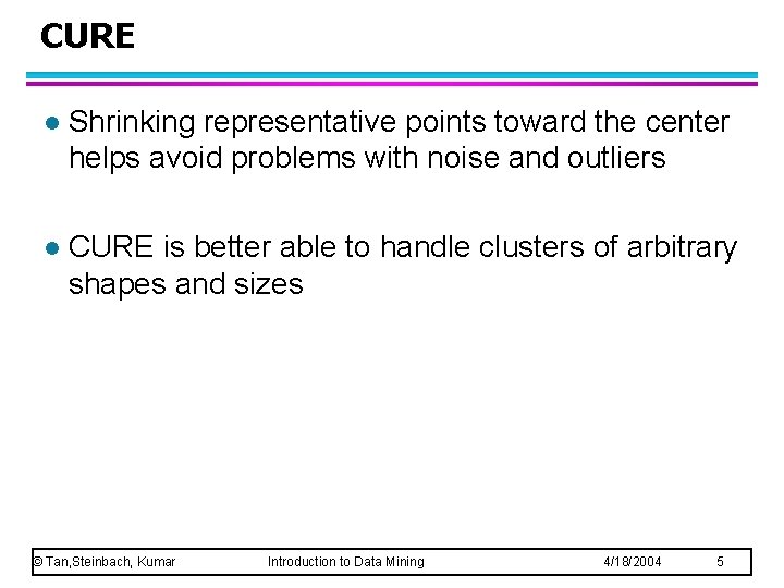
CURE l Shrinking representative points toward the center helps avoid problems with noise and outliers l CURE is better able to handle clusters of arbitrary shapes and sizes © Tan, Steinbach, Kumar Introduction to Data Mining 4/18/2004 5

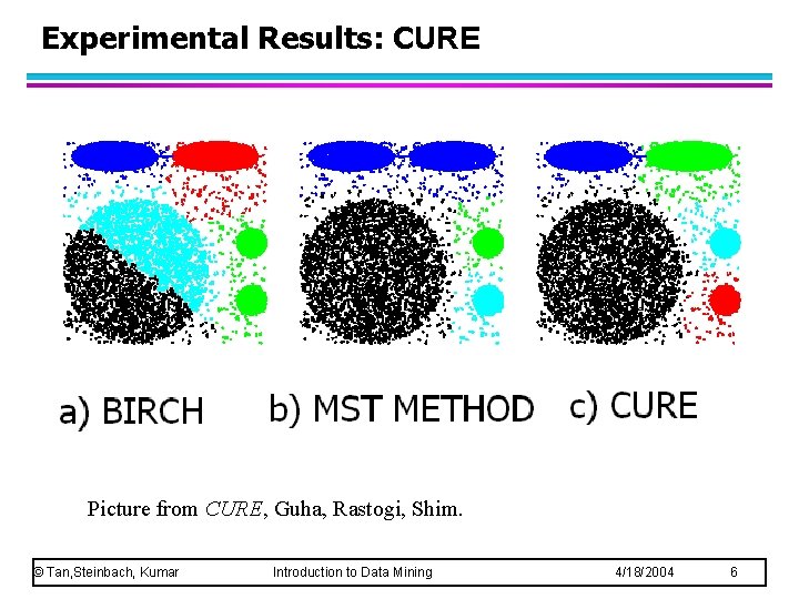
Experimental Results: CURE Picture from CURE, Guha, Rastogi, Shim. © Tan, Steinbach, Kumar Introduction to Data Mining 4/18/2004 6

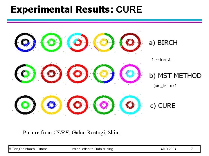
Experimental Results: CURE (centroid) (single link) Picture from CURE, Guha, Rastogi, Shim. © Tan, Steinbach, Kumar Introduction to Data Mining 4/18/2004 7

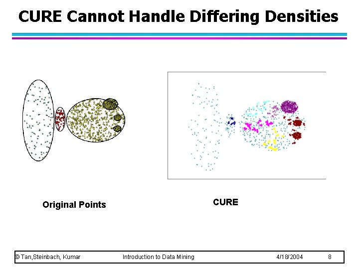
CURE Cannot Handle Differing Densities CURE Original Points © Tan, Steinbach, Kumar Introduction to Data Mining 4/18/2004 8

Graph-Based Clustering l Graph-Based clustering uses the proximity graph – Start with the proximity matrix – Consider each point as a node in a graph – Each edge between two nodes has a weight which is the proximity between the two points – Initially the proximity graph is fully connected – MIN (single-link) and MAX (complete-link) can be viewed as starting with this graph l In the simplest case, clusters are connected components in the graph. © Tan, Steinbach, Kumar Introduction to Data Mining 4/18/2004 9

Graph-Based Clustering: Sparsification l The amount of data that needs to be processed is drastically reduced – Sparsification can eliminate more than 99% of the entries in a proximity matrix – The amount of time required to cluster the data is drastically reduced – The size of the problems that can be handled is increased © Tan, Steinbach, Kumar Introduction to Data Mining 4/18/2004 10

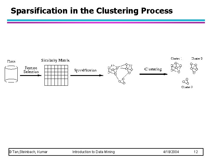
Graph-Based Clustering: Sparsification … l l Clustering may work better – Sparsification techniques keep the connections to the most similar (nearest) neighbors of a point while breaking the connections to less similar points. – The nearest neighbors of a point tend to belong to the same class as the point itself. – This reduces the impact of noise and outliers and sharpens the distinction between clusters. Sparsification facilitates the use of graph partitioning algorithms (or algorithms based on graph partitioning algorithms. – Chameleon and Hypergraph-based Clustering © Tan, Steinbach, Kumar Introduction to Data Mining 4/18/2004 11

Sparsification in the Clustering Process © Tan, Steinbach, Kumar Introduction to Data Mining 4/18/2004 12

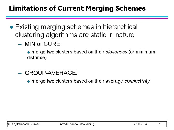
Limitations of Current Merging Schemes l Existing merging schemes in hierarchical clustering algorithms are static in nature – MIN or CURE: u merge two clusters based on their closeness (or minimum distance) – GROUP-AVERAGE: u merge two clusters based on their average connectivity © Tan, Steinbach, Kumar Introduction to Data Mining 4/18/2004 13

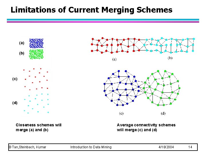
Limitations of Current Merging Schemes (a) (b) (c) (d) Closeness schemes will merge (a) and (b) © Tan, Steinbach, Kumar Average connectivity schemes will merge (c) and (d) Introduction to Data Mining 4/18/2004 14

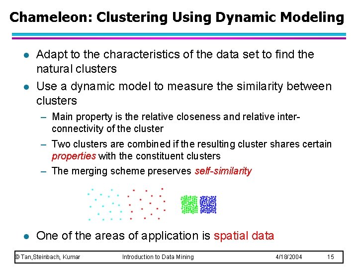
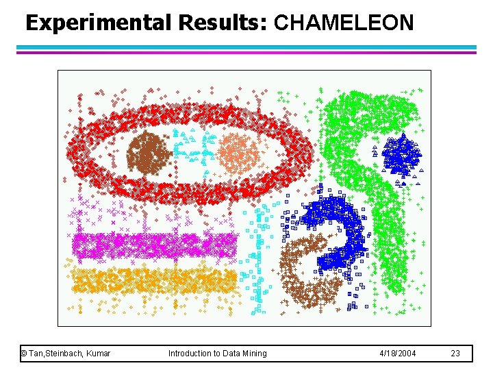
Chameleon: Clustering Using Dynamic Modeling l l Adapt to the characteristics of the data set to find the natural clusters Use a dynamic model to measure the similarity between clusters – Main property is the relative closeness and relative interconnectivity of the cluster – Two clusters are combined if the resulting cluster shares certain properties with the constituent clusters – The merging scheme preserves self-similarity l One of the areas of application is spatial data © Tan, Steinbach, Kumar Introduction to Data Mining 4/18/2004 15

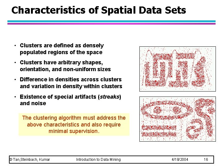
Characteristics of Spatial Data Sets • Clusters are defined as densely populated regions of the space • Clusters have arbitrary shapes, orientation, and non-uniform sizes • Difference in densities across clusters and variation in density within clusters • Existence of special artifacts (streaks) and noise The clustering algorithm must address the above characteristics and also require minimal supervision. © Tan, Steinbach, Kumar Introduction to Data Mining 4/18/2004 16

Chameleon: Steps l Preprocessing Step: Represent the Data by a Graph – Given a set of points, construct the k-nearest-neighbor (k-NN) graph to capture the relationship between a point and its k nearest neighbors – Concept of neighborhood is captured dynamically (even if region is sparse) l Phase 1: Use a multilevel graph partitioning algorithm on the graph to find a large number of clusters of well-connected vertices – Each cluster should contain mostly points from one “true” cluster, i. e. , is a sub-cluster of a “real” cluster © Tan, Steinbach, Kumar Introduction to Data Mining 4/18/2004 17

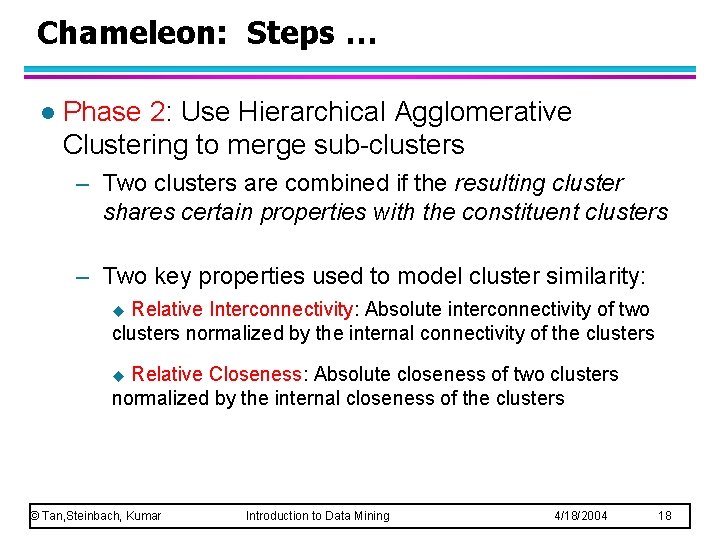
Chameleon: Steps … l Phase 2: Use Hierarchical Agglomerative Clustering to merge sub-clusters – Two clusters are combined if the resulting cluster shares certain properties with the constituent clusters – Two key properties used to model cluster similarity: u Relative Interconnectivity: Absolute interconnectivity of two clusters normalized by the internal connectivity of the clusters u Relative Closeness: Absolute closeness of two clusters normalized by the internal closeness of the clusters © Tan, Steinbach, Kumar Introduction to Data Mining 4/18/2004 18

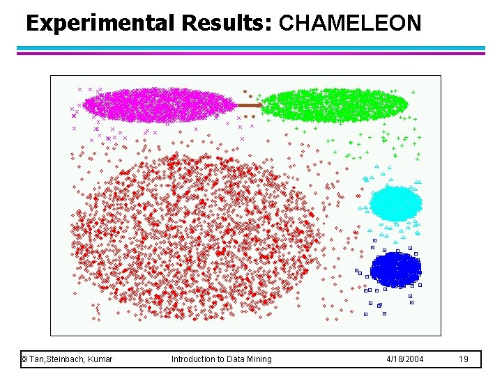
Experimental Results: CHAMELEON © Tan, Steinbach, Kumar Introduction to Data Mining 4/18/2004 19

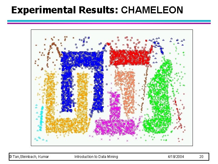
Experimental Results: CHAMELEON © Tan, Steinbach, Kumar Introduction to Data Mining 4/18/2004 20

Experimental Results: CURE (10 clusters) © Tan, Steinbach, Kumar Introduction to Data Mining 4/18/2004 21

Experimental Results: CURE (15 clusters) © Tan, Steinbach, Kumar Introduction to Data Mining 4/18/2004 22

Experimental Results: CHAMELEON © Tan, Steinbach, Kumar Introduction to Data Mining 4/18/2004 23

Experimental Results: CURE (9 clusters) © Tan, Steinbach, Kumar Introduction to Data Mining 4/18/2004 24

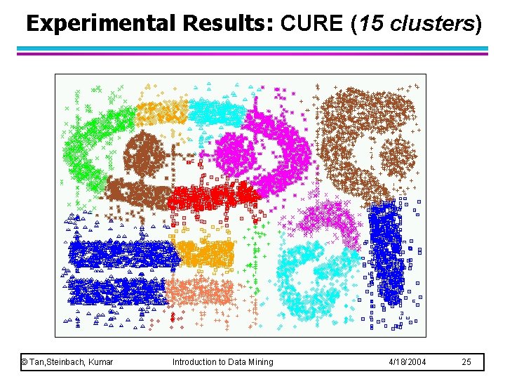
Experimental Results: CURE (15 clusters) © Tan, Steinbach, Kumar Introduction to Data Mining 4/18/2004 25

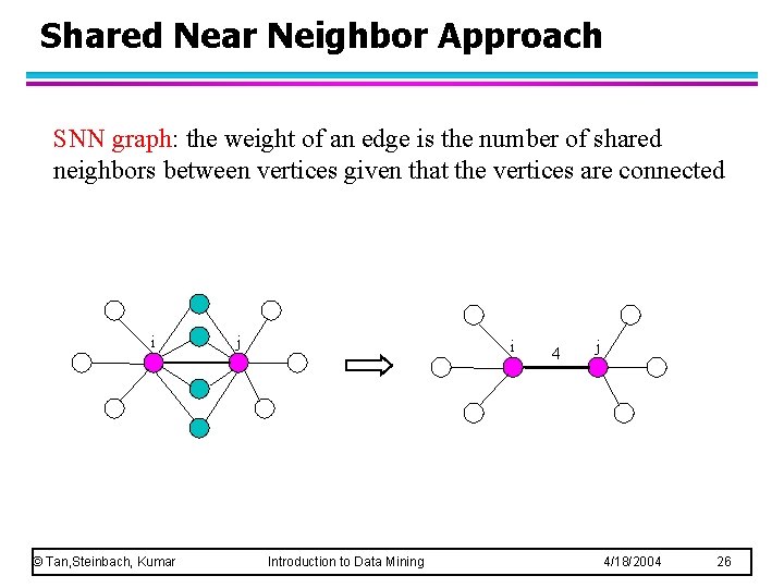
Shared Near Neighbor Approach SNN graph: the weight of an edge is the number of shared neighbors between vertices given that the vertices are connected i © Tan, Steinbach, Kumar j i Introduction to Data Mining 4 j 4/18/2004 26

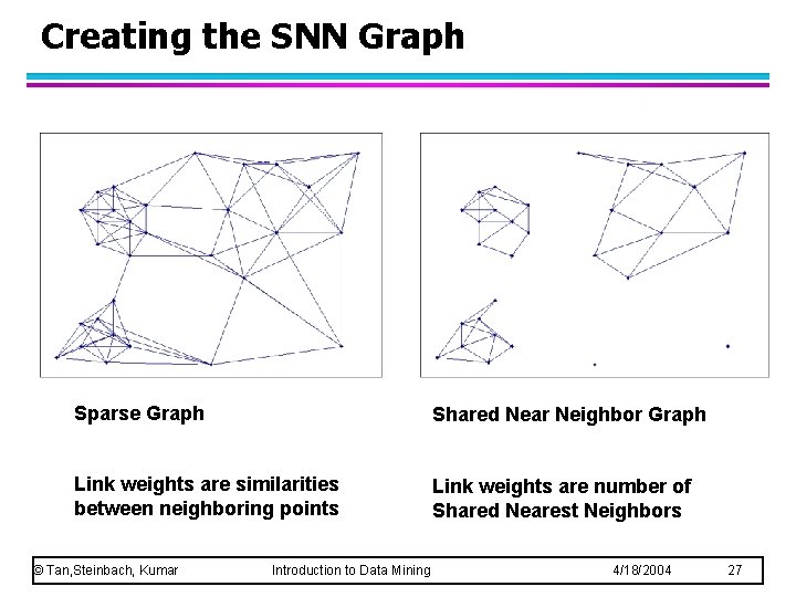
Creating the SNN Graph Sparse Graph Shared Near Neighbor Graph Link weights are similarities between neighboring points Link weights are number of Shared Nearest Neighbors © Tan, Steinbach, Kumar Introduction to Data Mining 4/18/2004 27

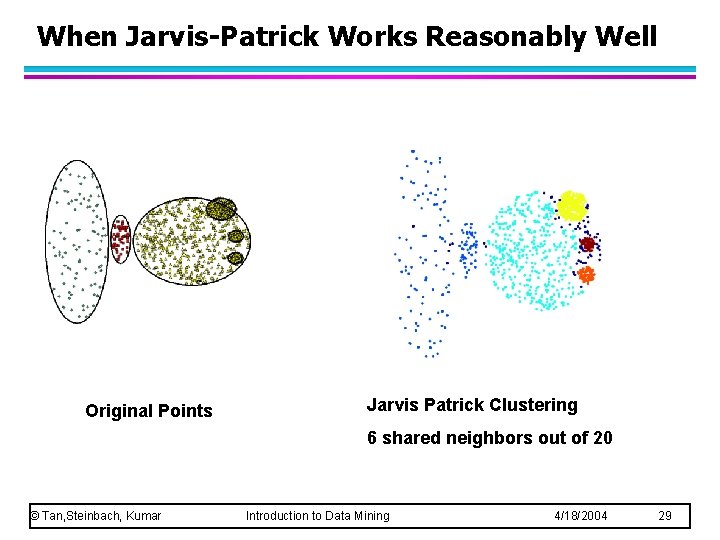
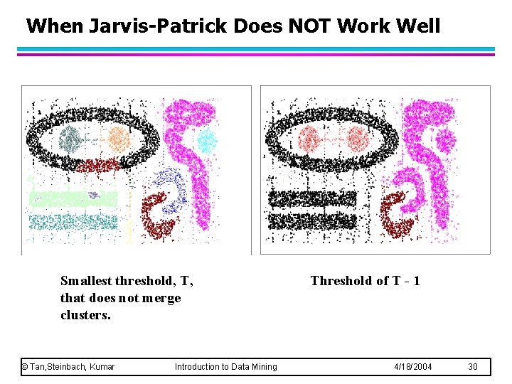
Jarvis-Patrick Clustering l First, the k-nearest neighbors of all points are found – In graph terms this can be regarded as breaking all but the k strongest links from a point to other points in the proximity graph l A pair of points is put in the same cluster if – any two points share more than T neighbors and – the two points are in each others k nearest neighbor list l For instance, we might choose a nearest neighbor list of size 20 and put points in the same cluster if they share more than 10 near neighbors © Tan, Steinbach, Kumar Introduction to Data Mining 4/18/2004 28

When Jarvis-Patrick Works Reasonably Well Original Points Jarvis Patrick Clustering 6 shared neighbors out of 20 © Tan, Steinbach, Kumar Introduction to Data Mining 4/18/2004 29

When Jarvis-Patrick Does NOT Work Well Smallest threshold, T, that does not merge clusters. © Tan, Steinbach, Kumar Introduction to Data Mining Threshold of T - 1 4/18/2004 30

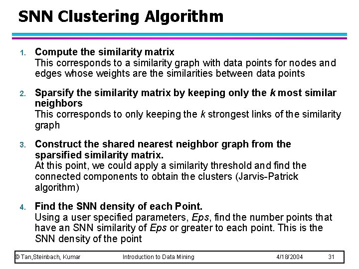
SNN Clustering Algorithm 1. Compute the similarity matrix This corresponds to a similarity graph with data points for nodes and edges whose weights are the similarities between data points 2. Sparsify the similarity matrix by keeping only the k most similar neighbors This corresponds to only keeping the k strongest links of the similarity graph 3. Construct the shared nearest neighbor graph from the sparsified similarity matrix. At this point, we could apply a similarity threshold and find the connected components to obtain the clusters (Jarvis-Patrick algorithm) 4. Find the SNN density of each Point. Using a user specified parameters, Eps, find the number points that have an SNN similarity of Eps or greater to each point. This is the SNN density of the point © Tan, Steinbach, Kumar Introduction to Data Mining 4/18/2004 31

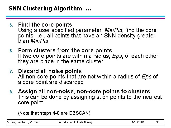
SNN Clustering Algorithm … 5. Find the core points Using a user specified parameter, Min. Pts, find the core points, i. e. , all points that have an SNN density greater than Min. Pts 6. Form clusters from the core points If two core points are within a radius, Eps, of each other they are place in the same cluster 7. Discard all noise points All non-core points that are not within a radius of Eps of a core point are discarded 8. Assign all non-noise, non-core points to clusters This can be done by assigning such points to the nearest core point (Note that steps 4 -8 are DBSCAN) © Tan, Steinbach, Kumar Introduction to Data Mining 4/18/2004 32

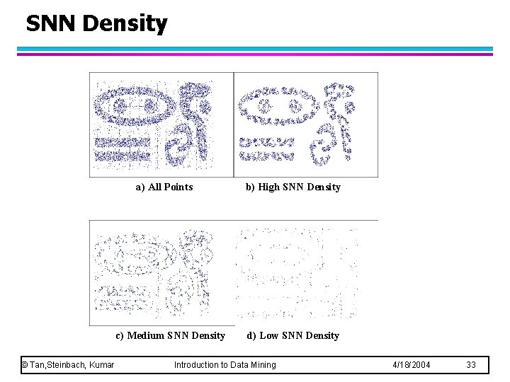
SNN Density a) All Points c) Medium SNN Density © Tan, Steinbach, Kumar b) High SNN Density d) Low SNN Density Introduction to Data Mining 4/18/2004 33

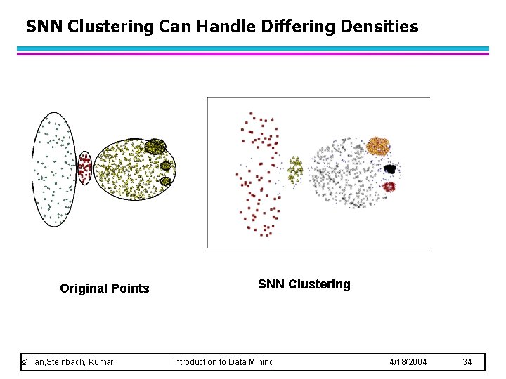
SNN Clustering Can Handle Differing Densities Original Points © Tan, Steinbach, Kumar SNN Clustering Introduction to Data Mining 4/18/2004 34

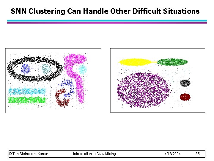
SNN Clustering Can Handle Other Difficult Situations © Tan, Steinbach, Kumar Introduction to Data Mining 4/18/2004 35

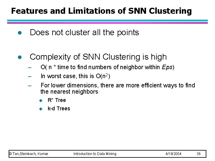
Features and Limitations of SNN Clustering l Does not cluster all the points l Complexity of SNN Clustering is high – – – O( n * time to find numbers of neighbor within Eps) In worst case, this is O(n 2) For lower dimensions, there are more efficient ways to find the nearest neighbors u R* Tree u k-d Trees © Tan, Steinbach, Kumar Introduction to Data Mining 4/18/2004 36