CLUSTER ANALYSIS CLUSTER ANALYSIS Cluster Analysis CA is

CLUSTER ANALYSIS

CLUSTER ANALYSIS • Cluster Analysis (CA) is an exploratory data analysis tool for organizing observed data (e. g. people, things, events, brands, companies) into meaningful taxonomies, groups, or clusters. • It is based on combinations of IV’s which maximizes the similarity of cases within each cluster while maximizing the dissimilarity between groups that are initially unknown.

CLUSTER ANALYSIS • CA creates new groupings without any preconceived notion of what clusters may arise whereas discriminant analysis classifies people and items into already known groups. • CA provides no explanation as to why the clusters exist nor is any interpretation made. Each cluster thus describes, in terms of the data collected, the class to which its members belong.

CLUSTER ANALYSIS Clustering occurs in almost every aspect of daily life. • A factory’s Health and Safety Committee may be regarded as a cluster of people. • Supermarkets display items of similar nature, such as types of meat or vegetables in the same or nearby locations. • Biologists have to organize the different species of animals before a meaningful description of the differences between animals is possible. • In medicine, the clustering of symptoms and diseases leads to taxonomies of illnesses. • In the field of business, clusters of consumer segments are often sought for successful marketing strategies.

BRANDING • Brand image analysis, or defining product "types" by customer perceptions, allows a company to see where its products are positioned in the market relative to those of its competitors. • This type of modelling is valuable for branding new products or identifying possible gaps in the market. • Clustering supermarket products by linked purchasing patterns can be used to plan store layouts, maximizing spontaneous purchasing opportunities.

Bank Example • Banking institutions have used hierarchical cluster analysis to develop a typology of customers, for two purposes, as follows: – To retain the loyalty of members by designing the best possible new financial products to meet the needs of different groups (clusters). – To capture more market share by identifying which existing services are most profitable for which type of customer and improve market penetration.

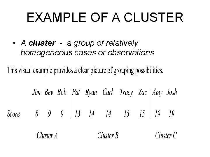
EXAMPLE OF A CLUSTER • A cluster - a group of relatively homogeneous cases or observations

USE OF CLUSTER ANALYSIS • You want to undertake direct mail advertising with specific advertisements for different groups of people. • You could use a variety of IV’s like family income, age, number of cars per family, number of mobile phones per family, number of school children per family etc… and different postal or zip codes characterized by particular combinations of demographic variables which could be grouped together to create a better way of directing the mail out. • You might in fact find that postal codes could be grouped into a number of clusters e. g. ‘the retirement zone’, ‘nappy valley’, ‘the golf club set’, the ‘rotweiler in a pickup’ district, etc. • This sort of grouping might also be valuable in deciding where to place several new wine stores, or ‘Tummy to Toddler’ shops.

USE OF CLUSTER ANALYSIS • Using cluster analysis, a customer "type" can represent a homogeneous market segment. Identifying their particular needs in that market allows products to be designed and advertising directed with greater precision and appeal within the segment. • Targeting specific segments is cheaper and more accurate than broad-scale marketing. • Customers respond better to segment marketing which addresses their specific needs, leading to increased market share and customer retention.

USE OF CLUSTER ANALYSIS • Imagine four clusters or market segments in the vacation travel industry. They are: (1) The elite - want top level service and expect to be pampered. (2) The escapists - want to get away and just relax. (3) The educationalist - wants to see new things, go to museums, have a safari, or experience new cultures. (4) The sports person - wants the golf course, tennis court, surfing, deep sea fishing, climbing, etc. • Different brochures and advertising is required for each of these.

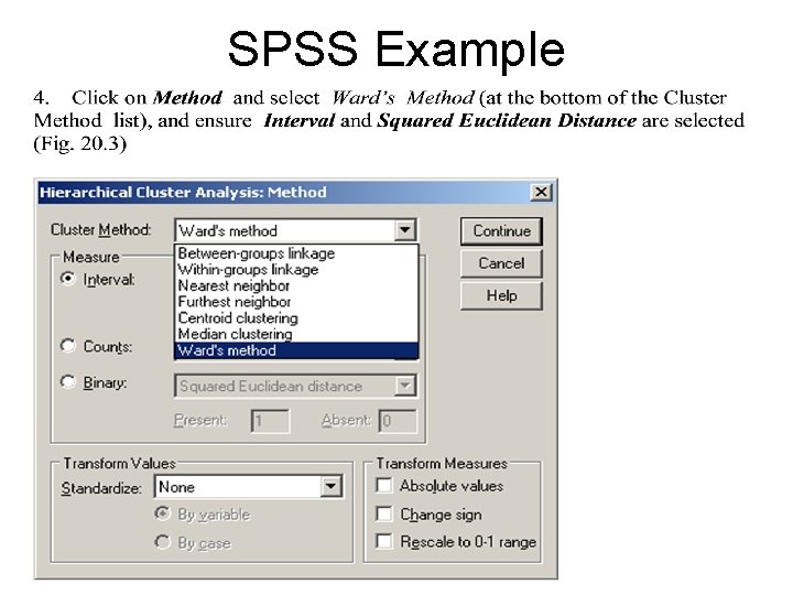
METHOD OF CLUSTER ANALYSIS Because we usually don’t know the number of groups or clusters that will emerge and because we want an optimum solution, a two-stage sequence of analysis occurs as follows. 1. We carry out a hierarchical cluster analysis using Ward’s method applying squared Euclidean Distance as the distance or similarity measure. This helps to determine the optimum number of clusters we should work with. 2. The next stage is to rerun the hierarchical cluster analysis with our selected number of clusters, which enables us to allocate every case in our sample to a particular cluster.

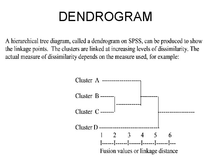
WARD’S METHOD • This is the major statistical method for finding relatively homogeneous clusters of cases based on measured characteristics. • It starts with each case as a separate cluster, i. e. there as many clusters as cases, and then combines the clusters sequentially, reducing the number of clusters at each step until only one cluster is left. • The clustering method uses the dissimilarities or distances between objects when forming the clusters. • The SPSS programme calculates ‘distances’ between data points in terms of the specified variables.

DENDROGRAM

Squared Euclidean Distance The most straightforward and generally accepted way of computing distances between objects in a multidimensional space is to compute Euclidean distances, an extension of Pythagorus’ theorem. In a univariate example, the Euclidean distance between two values is the arithmetic difference, i. e. value 1 value 2. In the bivariate case, the minimum distance is the hypotenuse of a triangle formed from the points as in Pythagoras’ theory. Although difficult to visualize, an extension of the Pythagoras’ theorem will also give the distance between two points in n-dimensional space.

Squared Euclidean Distance The squared Euclidean distance is used more often than the simple Euclidean distance in order to place progressively greater weight on objects that are further apart. Euclidean (and squared Euclidean) distances are usually computed from raw data, and not from standardized data.

WARD’S METHOD • SPSS provides five clustering algorithms, the most commonly used one being Ward’s method. Ward's method. This method is distinct from other methods because it uses analysis of variance to evaluate the distances between clusters. This method is very efficient. Cluster membership is assessed by calculating the total sum of squared deviations from the mean of a cluster. The criterion for fusion is that it should produce the smallest possible increase in the error sum of squares.

k-Means Clustering This method of clustering is very different from the hierarchical clustering and Ward method, which are applied when there is no prior knowledge of how many clusters there may be or what they are characterized by. K-means clustering is used when you already have hypotheses concerning the number of clusters in your cases or variables. You may want to "tell" the computer to form exactly 3 clusters that are to be as distinct as possible.

USE OF BOTH WARD AND KCLUSTERING • Very frequently, both the hierarchical and the kmeans techniques are used successively. • The former (Ward’s method) is used to get some sense of the possible number of clusters and the way they merge as seen from the dendrogram. • Then the clustering is rerun with only a chosen optimum number in which to place all the cases (k means clustering).

OPTIMUM NUMBER OF CLUSTERS • One of the biggest problems with cluster analysis is identifying the optimum number of clusters. • As the fusion process continues, increasingly dissimilar clusters must be fused, i. e. the classification becomes increasingly artificial. • Deciding upon the optimum number of clusters is largely subjective, although looking at a dendrogram may help.

SPSS EXAMPLE OF CLUSTER ANALYSIS • The data we will use includes 20 cases each responding to items on demographics (gender; qualifications, days absence from work, whether they smoke or not), on their attitudes to smoking in public places (subtest totals for pro and anti), plus total scale score for self concept. We are attempting to determine how many natural groups exist and who belongs to each group.

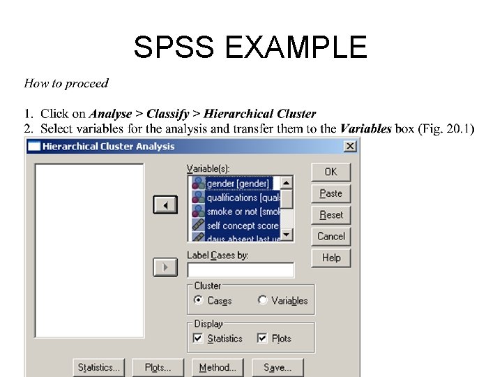
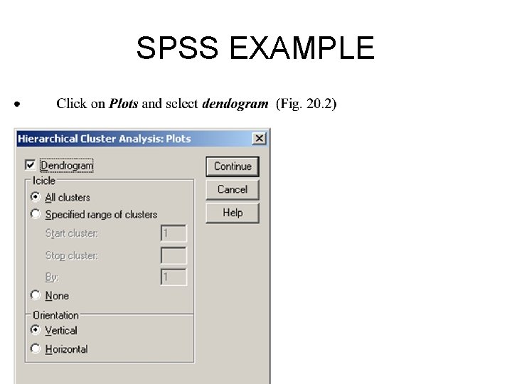
SPSS EXAMPLE • The initial step is determining how many groups exist. The SPSS hierarchical analysis actually calculates every possibility between everyone forming their own group (as many clusters as there are cases) and everyone belonging to the same group giving a range in our dummy set of data from 1 to 20 clusters.

SPSS EXAMPLE

SPSS EXAMPLE

SPSS Example

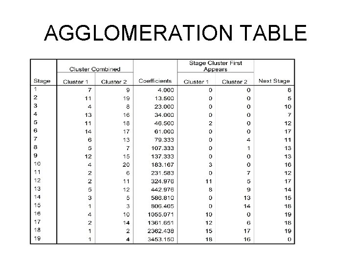
SPSS Example • 4. Select Continue then OK • The results start with an Agglomeration Table which provides a solution for every possible number of clusters from 1 to 20 (the number of our cases). The column to focus on is the central one which has the heading ‘Coefficients’. • Reading from the bottom upwards it shows that for one cluster we have an agglomeration coefficient of 3453. 150, for two clusters 2362. 438, for three clusters 1361. 651, etc.

AGGLOMERATION TABLE

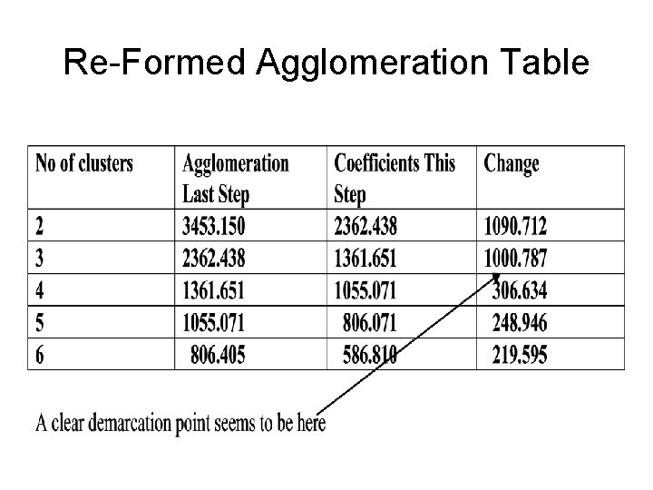
Reformed Agglomeration table • If we rewrite the coefficients as in the table in the next slide (not provided on SPSS) it is easier to see the changes in the coefficients as the number of clusters increase. • The final column headed ‘Change’ enables us to determine the optimum number of clusters. • In this case it is 3 clusters as succeeding clustering adds very much less to distinguishing between cases.

Re-Formed Agglomeration Table

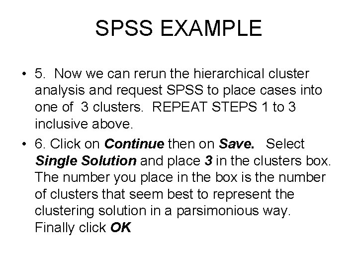
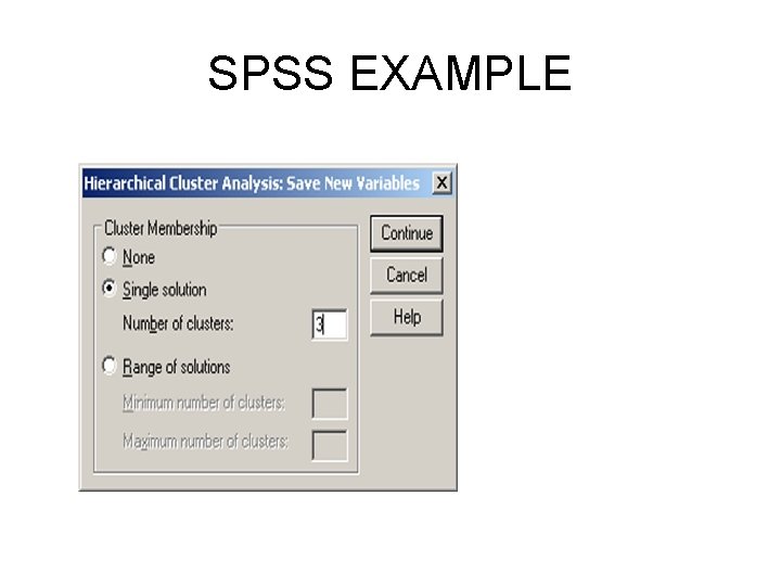
SPSS EXAMPLE • 5. Now we can rerun the hierarchical cluster analysis and request SPSS to place cases into one of 3 clusters. REPEAT STEPS 1 to 3 inclusive above. • 6. Click on Continue then on Save. Select Single Solution and place 3 in the clusters box. The number you place in the box is the number of clusters that seem best to represent the clustering solution in a parsimonious way. Finally click OK

SPSS EXAMPLE

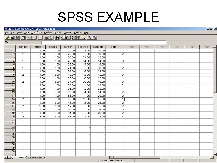
SPSS EXAMPLE • A new variable has been generated at the end of your SPSS data file called clu 3_1 (labeled Ward Method in variable view). • This provides the cluster membership for each case in your sample

SPSS EXAMPLE

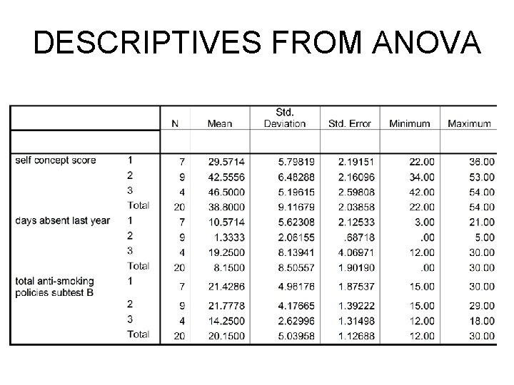
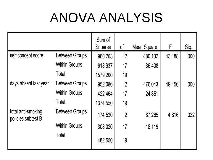
INTERPRETATION OF RESULTS • Nine respondents have been classified in cluster 2, while there are seven in cluster 1 and four in cluster 3. • As the result of a clustering analysis, we can examine the means for each cluster on each dimension using ANOVA to assess how distinct our clusters are. • Ideally, we would obtain significantly different means for most, if not all dimensions, used in the analysis. • The size of the F values performed on each dimension is an indication of how well the respective dimension discriminates between clusters.

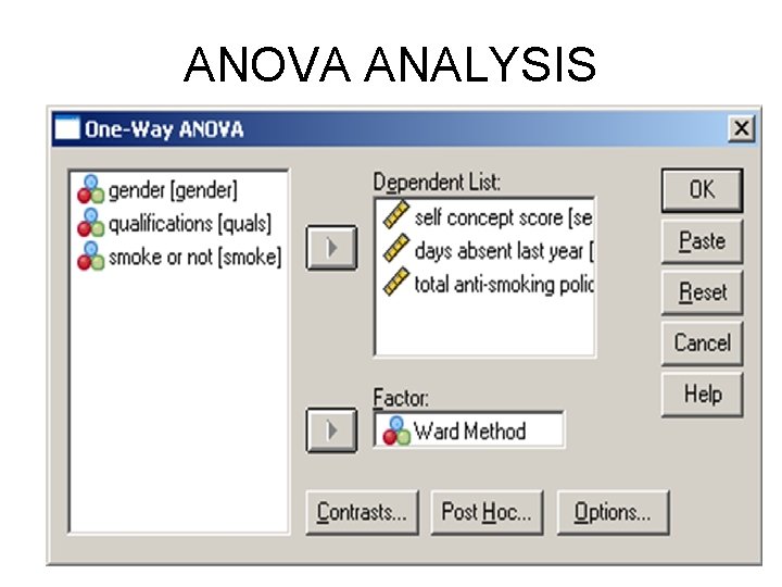
ARE CLUSTERS DISTINCT? • In conducting the one way ANOVA, you can produce the descriptives on the scale (interval) variables for each of the clusters and note the differences. • The grouping variable is the new clusters variable. • Categorical (nominal) data can be dealt with using Crosstabs • The One Way ANOVA box and descriptives table are shown next.

ANOVA ANALYSIS

DESCRIPTIVES FROM ANOVA

ANOVA ANALYSIS

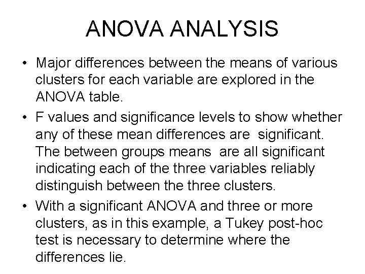
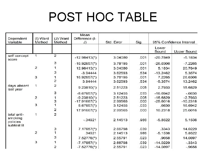
ANOVA ANALYSIS • Major differences between the means of various clusters for each variable are explored in the ANOVA table. • F values and significance levels to show whether any of these mean differences are significant. The between groups means are all significant indicating each of the three variables reliably distinguish between the three clusters. • With a significant ANOVA and three or more clusters, as in this example, a Tukey post-hoc test is necessary to determine where the differences lie.

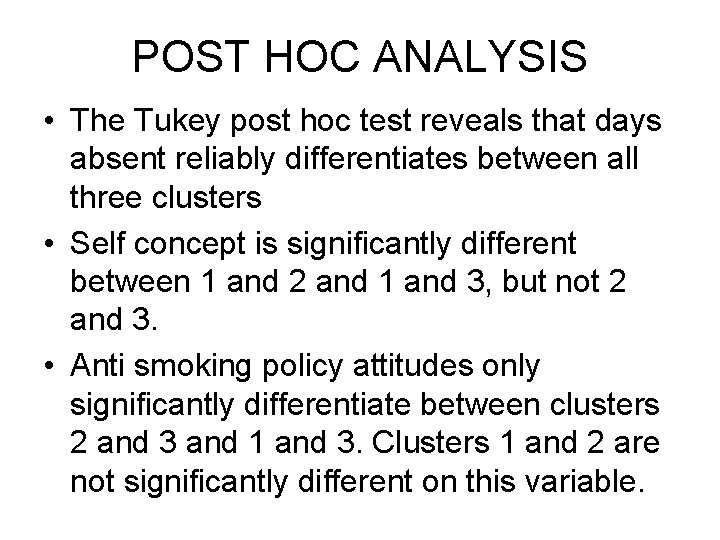
POST HOC ANALYSIS • The Tukey post hoc test reveals that days absent reliably differentiates between all three clusters • Self concept is significantly different between 1 and 2 and 1 and 3, but not 2 and 3. • Anti smoking policy attitudes only significantly differentiate between clusters 2 and 3 and 1 and 3. Clusters 1 and 2 are not significantly different on this variable.

POST HOC TABLE

CROSS TAB ANALYSIS • Crosstab analysis of nominal variables gender, qualifications and whether smoke or not produced some significant associations with clusters. • Of course, with such small numbers we would not normally have conducted a crosstabs as many cells would have counts less than 5. This explanation has been solely to show you can tease out the characteristics of the clusters.

CROSS TAB ANALYSIS • The three clusters significantly differentiated between gender with males in clusters 1 and 2 and females in 3. • Smoking also produced significant associations with non-smokers in cluster 1 and smokers in 3. • Cluster 2 represented both smokers and nonsmokers who were differentiated by other variables. • Qualifications did not produce any significant associations. • Histograms can be produced with the crosstabs analysis to reveal useful visual differentiations of the groupings

SUMMARY OF RESULTS • When Cluster memberships are significantly different they can be used as a new grouping variable in other analyses. • In our example: – Cluster 1 is characterized by low self concept, average absence rate, average attitude score to anti smoking, and nonsmoking males – Cluster 2 is characterized by moderate self concept, low absence rate, average attitude score to anti smoking, with both smoking and nonsmoking males. – Cluster 3 is characterized by high self concept, high absence rate, low score to anti smoking, and smoking females • It is important to remember that cluster analysis will always produce a grouping - these may or may not prove useful for classifying items.