Introduction to Graph Cluster Analysis Outline Introduction to

Introduction to Graph Cluster Analysis

Outline • Introduction to Cluster Analysis • Types of Graph Cluster Analysis • Algorithms for Graph Clustering q k-Spanning Tree q Shared Nearest Neighbor q Betweenness Centrality Based q Highly Connected Components q Maximal Clique Enumeration q Kernel k-means • Application 2

Outline • Introduction to Clustering • Introduction to Graph Clustering • Algorithms for Graph Clustering q k-Spanning Tree q Shared Nearest Neighbor q Betweenness Centrality Based q Highly Connected Components q Maximal Clique Enumeration q Kernel k-means • Application 3

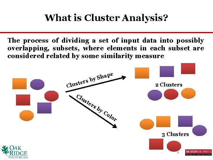
What is Cluster Analysis? The process of dividing a set of input data into possibly overlapping, subsets, where elements in each subset are considered related by some similarity measure rs e t s Clu Cl pe ha S y b us te 2 Clusters rs b y. C ol or 3 Clusters 4

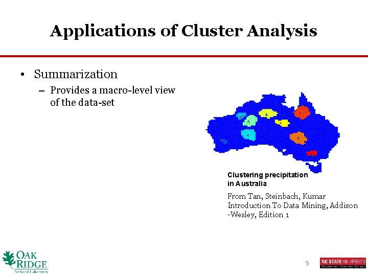
Applications of Cluster Analysis • Summarization – Provides a macro-level view of the data-set Clustering precipitation in Australia From Tan, Steinbach, Kumar Introduction To Data Mining, Addison -Wesley, Edition 1 5

Outline • Introduction to Clustering • Introduction to Graph Clustering • Algorithms for Graph Clustering q k-Spanning Tree q Shared Nearest Neighbor q Betweenness Centrality Based q Highly Connected Components q Maximal Clique Enumeration q Kernel k-means • Application 6

What is Graph Clustering? • Types – Between-graph • Clustering a set of graphs – Within-graph • Clustering the nodes/edges of a single graph 7

Between-graph Clustering Between-graph clustering methods divide a set of graphs into different clusters E. g. , A set of graphs representing chemical compounds can be grouped into clusters based on their structural similarity 8

Within-graph Clustering Within-graph clustering methods divides the nodes of a graph into clusters E. g. , In a social networking graph, these clusters could represent people with same/similar hobbies Note: In this chapter we will look at different algorithms to perform within-graph clustering 9

Outline • Introduction to Clustering • Introduction to Graph Clustering • Algorithms for Within Graph Clustering q k-Spanning Tree q Shared Nearest Neighbor q Betweenness Centrality Based q Highly Connected Components q Maximal Clique Enumeration q Kernel k-means • Application 10

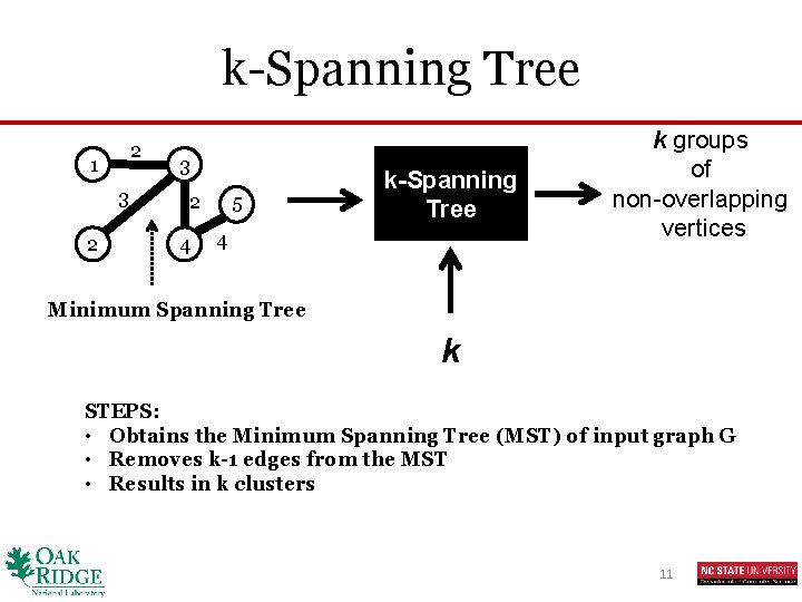
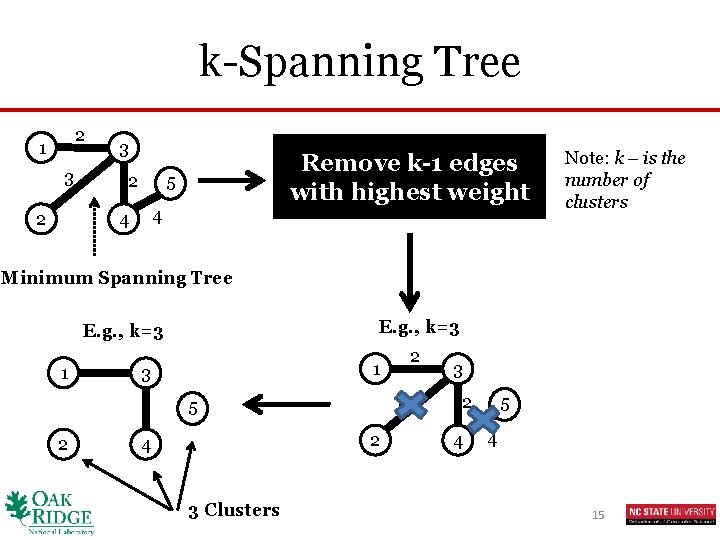
k-Spanning Tree 2 1 3 2 4 5 k-Spanning Tree 4 k groups of non-overlapping vertices Minimum Spanning Tree k STEPS: • Obtains the Minimum Spanning Tree (MST) of input graph G • Removes k-1 edges from the MST • Results in k clusters 11

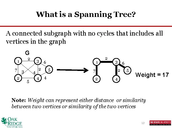
What is a Spanning Tree? A connected subgraph with no cycles that includes all vertices in the graph G 2 1 7 3 2 3 4 5 2 4 1 6 5 4 2 3 6 2 7 2 4 5 Weight = 17 Note: Weight can represent either distance or similarity between two vertices or similarity of the two vertices 12

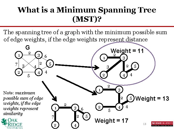
What is a Minimum Spanning Tree (MST)? The spanning tree of a graph with the minimum possible sum of edge weights, if the edge weights represent distance G Weight = 11 2 2 3 1 7 3 2 4 5 6 2 4 Note: maximum possible sum of edge weights, if the edge weights represent similarity 3 1 5 2 3 4 2 1 4 4 2 3 2 1 2 3 2 7 2 4 2 6 5 5 5 4 5 Weight = 13 4 Weight = 17 13

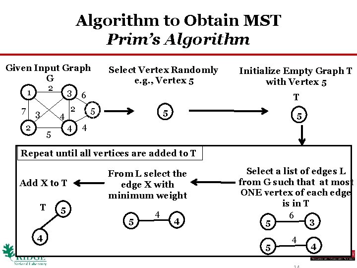
Algorithm to Obtain MST Prim’s Algorithm Given Input Graph G 2 3 6 1 7 3 2 2 4 4 5 Select Vertex Randomly e. g. , Vertex 5 Initialize Empty Graph T with Vertex 5 T 5 5 5 4 Repeat until all vertices are added to T Add X to T T From L select the edge X with minimum weight 5 5 4 4 4 Select a list of edges L from G such that at most ONE vertex of each edge is in T 6 3 5 5 4 4

k-Spanning Tree 2 1 3 2 Remove k-1 edges with highest weight 5 4 4 Note: k – is the number of clusters Minimum Spanning Tree E. g. , k=3 1 3 3 5 2 2 1 2 4 3 Clusters 3 2 4 5 4 15

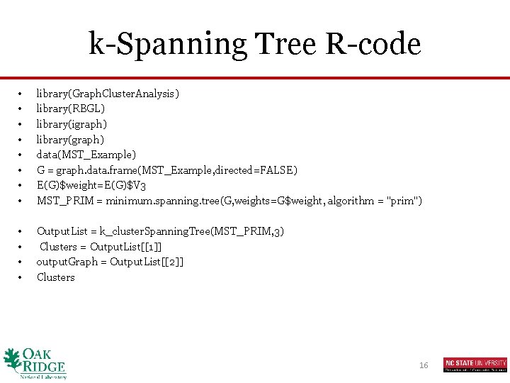
k-Spanning Tree R-code • • library(Graph. Cluster. Analysis) library(RBGL) library(igraph) library(graph) data(MST_Example) G = graph. data. frame(MST_Example, directed=FALSE) E(G)$weight=E(G)$V 3 MST_PRIM = minimum. spanning. tree(G, weights=G$weight, algorithm = "prim") • • Output. List = k_cluster. Spanning. Tree(MST_PRIM, 3) Clusters = Output. List[[1]] output. Graph = Output. List[[2]] Clusters 16

Outline • Introduction to Clustering • Introduction to Graph Clustering • Algorithms for Within Graph Clustering q k-Spanning Tree q Shared Nearest Neighbor Clustering q Betweenness Centrality Based q Highly Connected Components q Maximal Clique Enumeration q Kernel k-means • Application 17

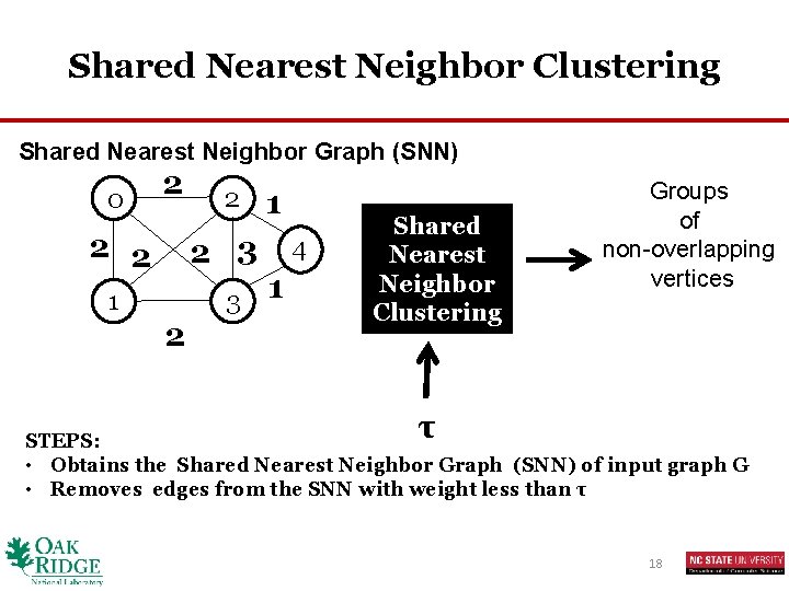
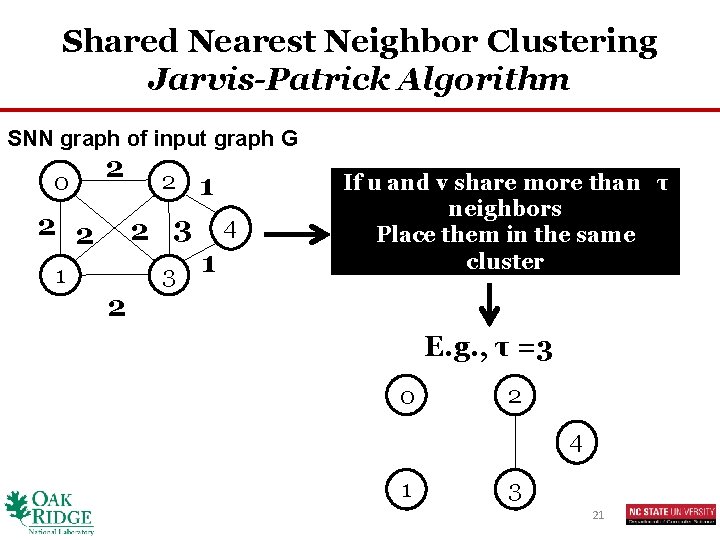
Shared Nearest Neighbor Clustering Shared Nearest Neighbor Graph (SNN) 0 2 2 2 1 2 2 3 1 4 1 Shared Nearest Neighbor Clustering Groups of non-overlapping vertices τ STEPS: • Obtains the Shared Nearest Neighbor Graph (SNN) of input graph G • Removes edges from the SNN with weight less than τ 18

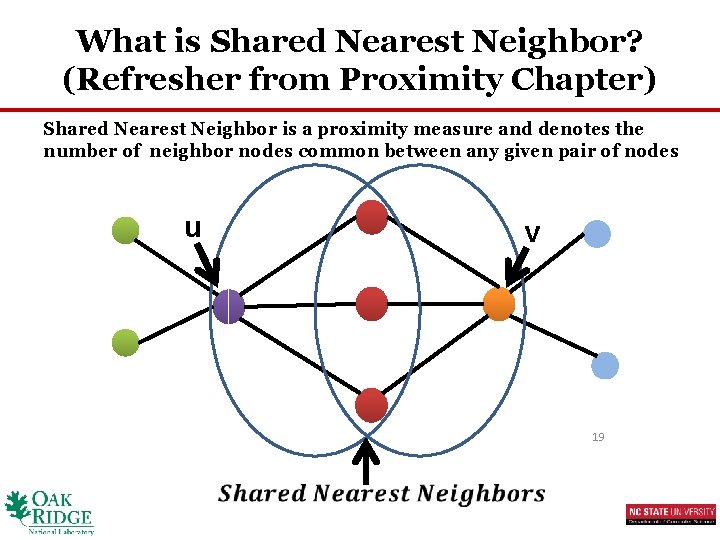
What is Shared Nearest Neighbor? (Refresher from Proximity Chapter) Shared Nearest Neighbor is a proximity measure and denotes the number of neighbor nodes common between any given pair of nodes u v 19

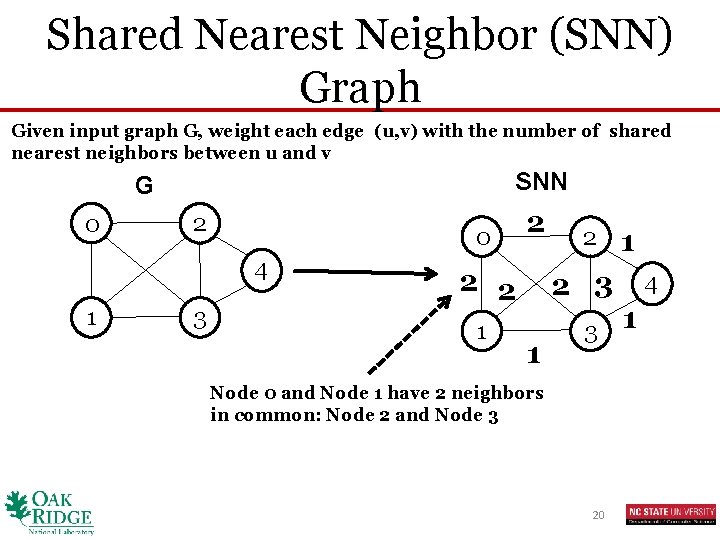
Shared Nearest Neighbor (SNN) Graph Given input graph G, weight each edge (u, v) with the number of shared nearest neighbors between u and v SNN G 0 2 0 4 1 3 2 2 2 1 2 2 3 1 3 Node 0 and Node 1 have 2 neighbors in common: Node 2 and Node 3 20 1 4 1

Shared Nearest Neighbor Clustering Jarvis-Patrick Algorithm SNN graph of input graph G 0 2 2 2 1 2 2 3 1 4 1 If u and v share more than τ neighbors Place them in the same cluster E. g. , τ =3 0 2 4 1 3 21

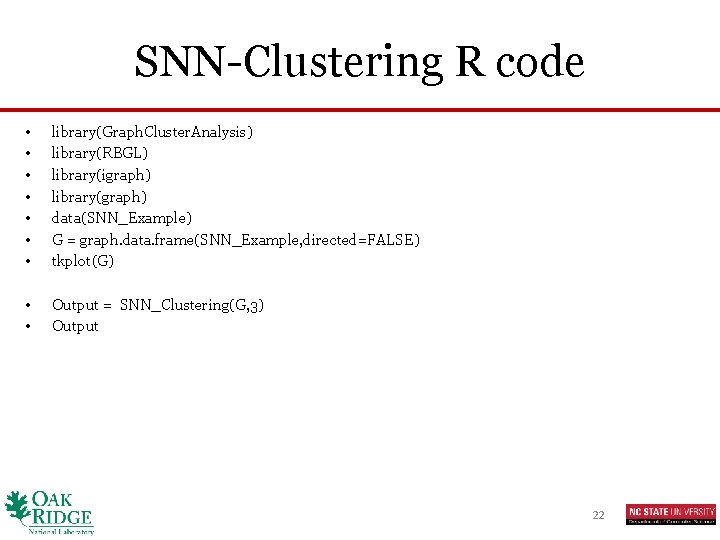
SNN-Clustering R code • • library(Graph. Cluster. Analysis) library(RBGL) library(igraph) library(graph) data(SNN_Example) G = graph. data. frame(SNN_Example, directed=FALSE) tkplot(G) • • Output = SNN_Clustering(G, 3) Output 22

Outline • Introduction to Clustering • Introduction to Graph Clustering • Algorithms for Within Graph Clustering q k-Spanning Tree q Shared Nearest Neighbor Clustering q Betweenness Centrality Based q Highly Connected Components q Maximal Clique Enumeration q Kernel k-means • Application 23

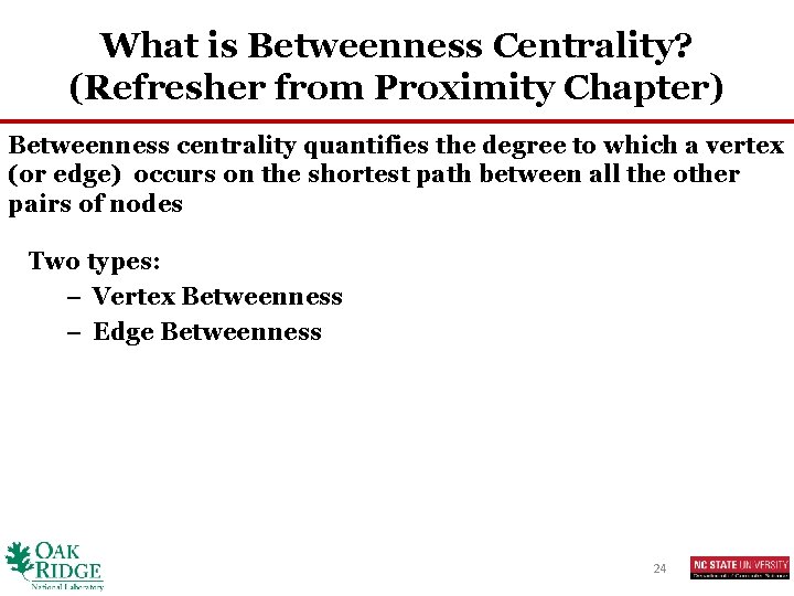
What is Betweenness Centrality? (Refresher from Proximity Chapter) Betweenness centrality quantifies the degree to which a vertex (or edge) occurs on the shortest path between all the other pairs of nodes Two types: – Vertex Betweenness – Edge Betweenness 24

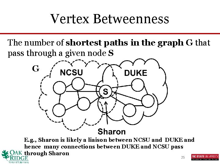
Vertex Betweenness The number of shortest paths in the graph G that pass through a given node S G E. g. , Sharon is likely a liaison between NCSU and DUKE and hence many connections between DUKE and NCSU pass through Sharon 25

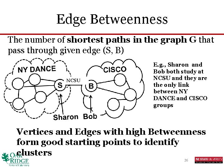
Edge Betweenness The number of shortest paths in the graph G that pass through given edge (S, B) NCSU E. g. , Sharon and Bob both study at NCSU and they are the only link between NY DANCE and CISCO groups Vertices and Edges with high Betweenness form good starting points to identify clusters 26

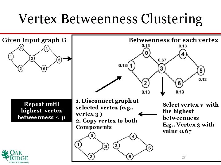
Vertex Betweenness Clustering Given Input graph G Repeat until highest vertex betweenness ≤ μ Betweenness for each vertex 1. Disconnect graph at selected vertex (e. g. , vertex 3 ) 2. Copy vertex to both Components Select vertex v with the highest betweenness E. g. , Vertex 3 with value 0. 67 27

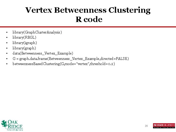
Vertex Betweenness Clustering R code • • library(Graph. Cluster. Analysis) library(RBGL) library(igraph) library(graph) data(Betweenness_Vertex_Example) G = graph. data. frame(Betweenness_Vertex_Example, directed=FALSE) betweenness. Based. Clustering(G, mode="vertex", threshold=0. 2) 28

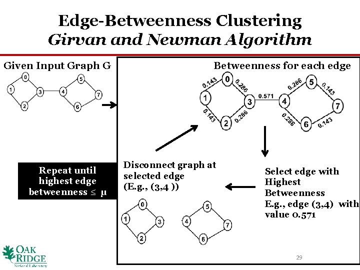
Edge-Betweenness Clustering Girvan and Newman Algorithm Given Input Graph G Repeat until highest edge betweenness ≤ μ Betweenness for each edge Disconnect graph at selected edge (E. g. , (3, 4 )) Select edge with Highest Betweenness E. g. , edge (3, 4) with value 0. 571 29

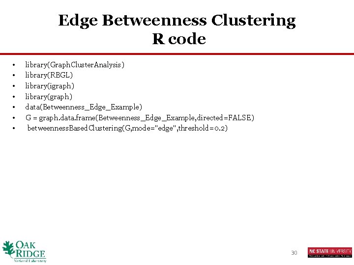
Edge Betweenness Clustering R code • • library(Graph. Cluster. Analysis) library(RBGL) library(igraph) library(graph) data(Betweenness_Edge_Example) G = graph. data. frame(Betweenness_Edge_Example, directed=FALSE) betweenness. Based. Clustering(G, mode="edge", threshold=0. 2) 30

Outline • Introduction to Clustering • Introduction to Graph Clustering • Algorithms for Within Graph Clustering q k-Spanning Tree q Shared Nearest Neighbor Clustering q Betweenness Centrality Based q Highly Connected Components q Maximal Clique Enumeration q Kernel k-means • Application 31

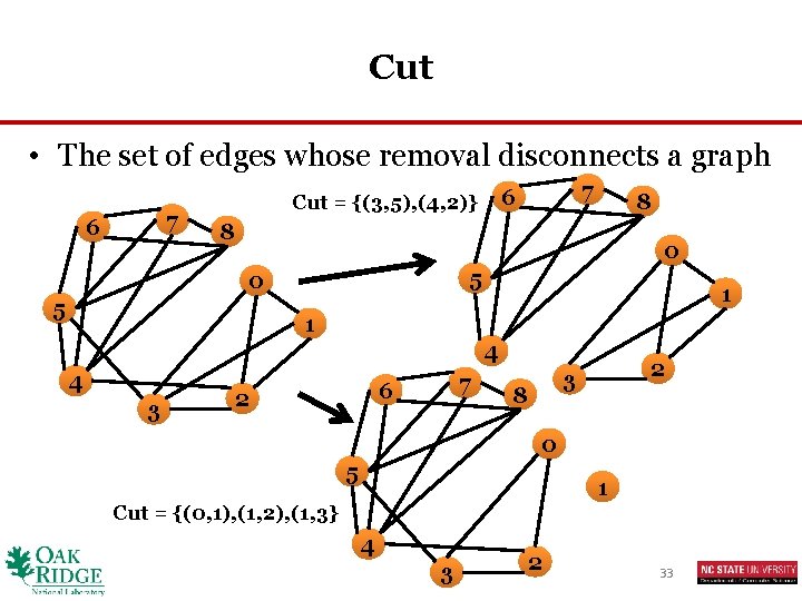
What is a Highly Connected Subgraph? • Requires the following definitions – Cut – Minimum Edge Cut (Min. Cut) – Edge Connectivity (EC) 32

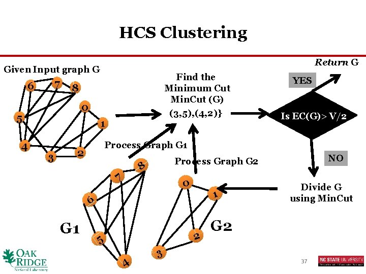
Cut • The set of edges whose removal disconnects a graph 7 6 Cut = {(3, 5), (4, 2)} 8 8 0 5 1 1 4 4 3 7 6 2 2 3 8 0 5 1 Cut = {(0, 1), (1, 2), (1, 3} 4 3 2 33

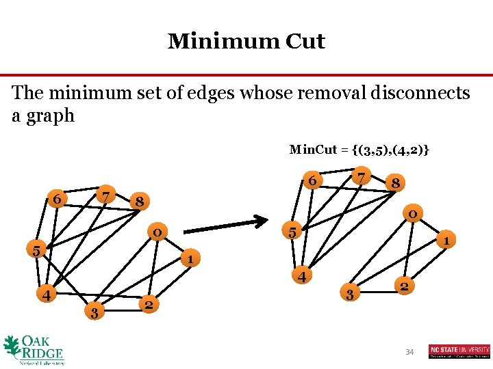
Minimum Cut The minimum set of edges whose removal disconnects a graph Min. Cut = {(3, 5), (4, 2)} 7 6 8 8 0 5 1 1 4 4 3 2 34

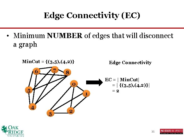
Edge Connectivity (EC) • Minimum NUMBER of edges that will disconnect a graph Min. Cut = {(3, 5), (4, 2)} 7 6 Edge Connectivity 8 0 5 1 4 3 EC = | Min. Cut| = | {(3, 5), (4, 2)}| =2 2 35

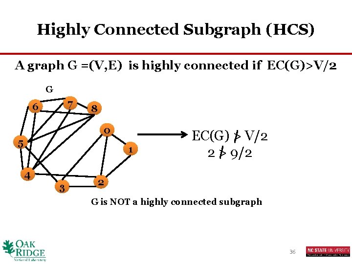
Highly Connected Subgraph (HCS) A graph G =(V, E) is highly connected if EC(G)>V/2 G 7 6 8 0 5 1 4 3 EC(G) > V/2 2 > 9/2 2 G is NOT a highly connected subgraph 36

HCS Clustering Return G Given Input graph G 7 6 8 0 5 4 Find the Minimum Cut Min. Cut (G) (3, 5), (4, 2)} 1 3 Is EC(G)> V/2 Process Graph G 1 2 0 1 6 2 5 4 NO Process Graph G 2 8 7 G 1 YES 3 Divide G using Min. Cut G 2 37

HCS Clustering R code • • library(Graph. Cluster. Analysis) library(RBGL) library(igraph) library(graph) data(HCS_Example) G = graph. data. frame(HCS_Example, directed=FALSE) HCSClustering(G, kappa=2) 38

Outline • Introduction to Clustering • Introduction to Graph Clustering • Algorithms for Within Graph Clustering q k-Spanning Tree q Shared Nearest Neighbor Clustering q Betweenness Centrality Based q Highly Connected Components q Maximal Clique Enumeration q Kernel k-means • Application 39

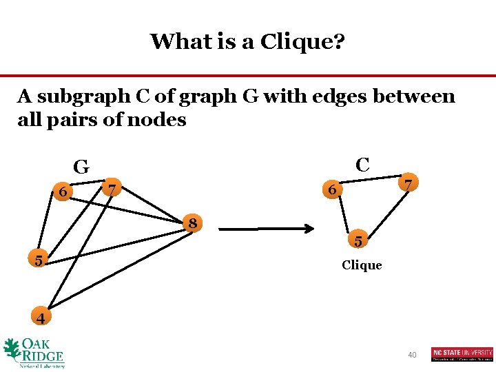
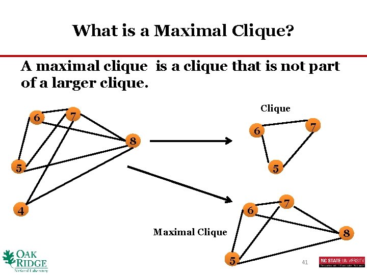
What is a Clique? A subgraph C of graph G with edges between all pairs of nodes C G 6 7 6 8 5 7 5 Clique 4 40

What is a Maximal Clique? A maximal clique is a clique that is not part of a larger clique. 6 Clique 7 7 6 8 5 5 4 6 7 Maximal Clique 8 5 41

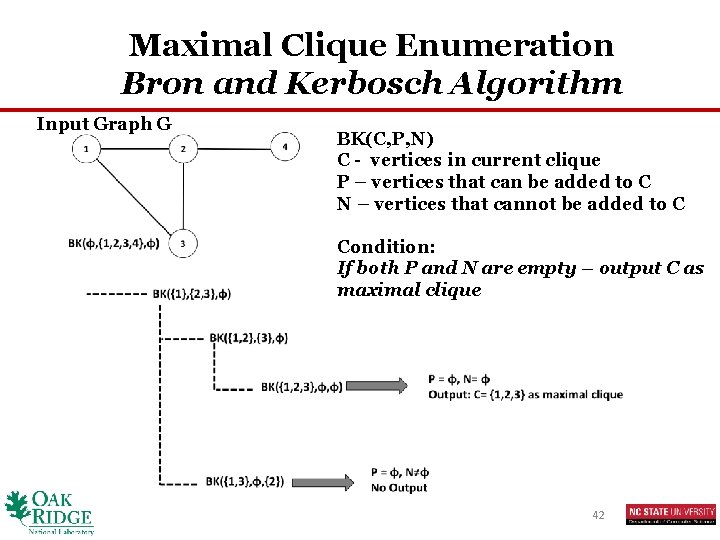
Maximal Clique Enumeration Bron and Kerbosch Algorithm Input Graph G BK(C, P, N) C - vertices in current clique P – vertices that can be added to C N – vertices that cannot be added to C Condition: If both P and N are empty – output C as maximal clique 42

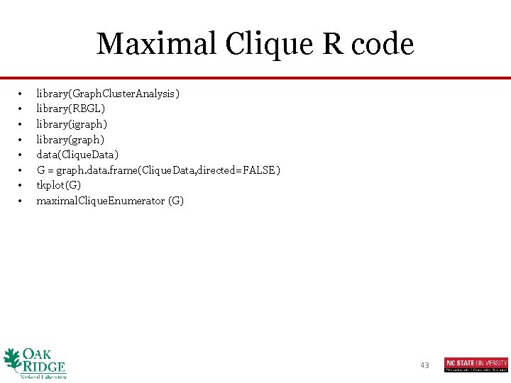
Maximal Clique R code • • library(Graph. Cluster. Analysis) library(RBGL) library(igraph) library(graph) data(Clique. Data) G = graph. data. frame(Clique. Data, directed=FALSE) tkplot(G) maximal. Clique. Enumerator (G) 43

Outline • Introduction to Clustering • Introduction to Graph Clustering • Algorithms for Within Graph Clustering q k-Spanning Tree q Shared Nearest Neighbor Clustering q Betweenness Centrality Based q Highly Connected Components q Maximal Clique Enumeration q Kernel k-means • Application 44

What is k-means? • k-means is a clustering algorithm applied to vector data points • k-means recap: – Select k data points from input as centroids 1. Assign other data points to the nearest centroid 2. Recompute centroid for each cluster 3. Repeat Steps 1 and 2 until centroids don’t change 45

k-means on Graphs Kernel K-means • Basic algorithm is the same as k-means on Vector data • We utilize the “kernel trick” (recall Kernel Chapter) • “kernel trick” recap – We know that we can use within-graph kernel functions to calculate the inner product of a pair of vertices in a userdefined feature space. – We replace the standard distance/proximity measures used in k-means with this within-graph kernel function 46

Outline • Introduction to Clustering • Introduction to Graph Clustering • Algorithms for Within Graph Clustering q k-Spanning Tree q Shared Nearest Neighbor Clustering q Betweenness Centrality Based q Highly Connected Components q Maximal Clique Enumeration q Kernel k-means • Application 47

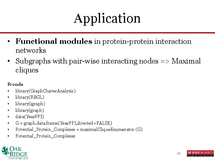
Application • Functional modules in protein-protein interaction networks • Subgraphs with pair-wise interacting nodes => Maximal cliques R-code • library(Graph. Cluster. Analysis) • library(RBGL) • library(igraph) • library(graph) • data(Yeas. PPI) • G = graph. data. frame(Yeas. PPI, directed=FALSE) • Potential_Protein_Complexes = maximal. Clique. Enumerator (G) • Potential_Protein_Complexes 48