Cluster Analysis Cluster Analysis p What is Cluster

Cluster Analysis

Cluster Analysis p What is Cluster Analysis? p Types of Data in Cluster Analysis p A Categorization of Major Clustering Methods p Partitioning Methods p Hierarchical Methods p Density-Based Methods p Grid-Based Methods p Model-Based Clustering Methods p Outlier Analysis p Summary

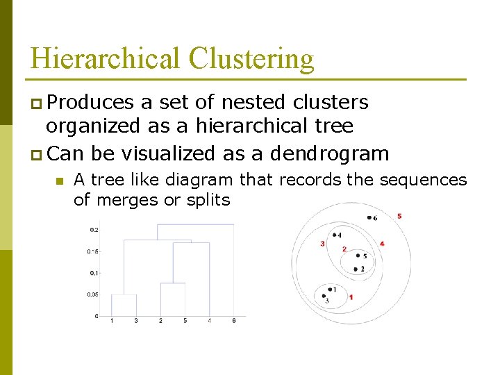
Hierarchical Clustering p Produces a set of nested clusters organized as a hierarchical tree p Can be visualized as a dendrogram n A tree like diagram that records the sequences of merges or splits

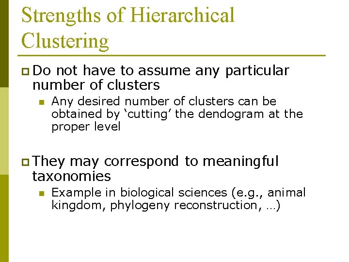
Strengths of Hierarchical Clustering p Do not have to assume any particular number of clusters n Any desired number of clusters can be obtained by ‘cutting’ the dendogram at the proper level p They may correspond to meaningful taxonomies n Example in biological sciences (e. g. , animal kingdom, phylogeny reconstruction, …)

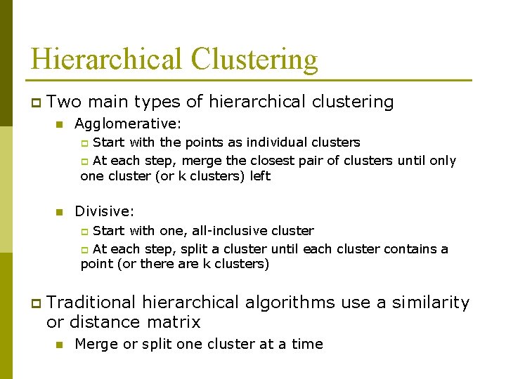
Hierarchical Clustering p Two main types of hierarchical clustering n Agglomerative: Start with the points as individual clusters p At each step, merge the closest pair of clusters until only one cluster (or k clusters) left p n Divisive: Start with one, all-inclusive cluster p At each step, split a cluster until each cluster contains a point (or there are k clusters) p p Traditional hierarchical algorithms use a similarity or distance matrix n Merge or split one cluster at a time

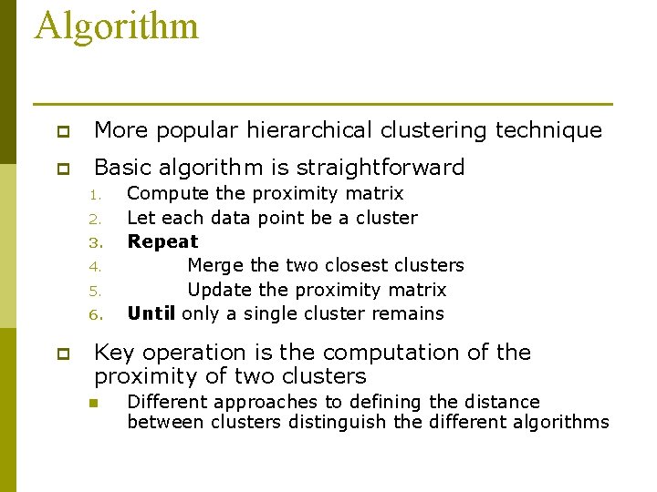
Algorithm p More popular hierarchical clustering technique p Basic algorithm is straightforward 1. 2. 3. 4. 5. 6. p Compute the proximity matrix Let each data point be a cluster Repeat Merge the two closest clusters Update the proximity matrix Until only a single cluster remains Key operation is the computation of the proximity of two clusters n Different approaches to defining the distance between clusters distinguish the different algorithms

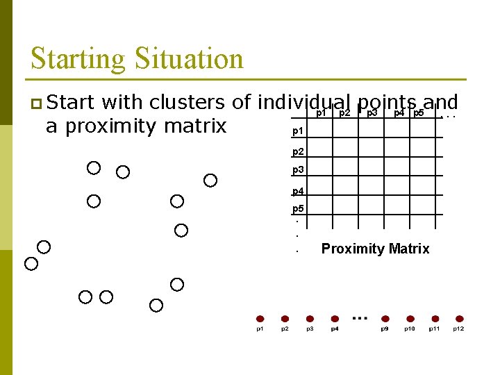
Starting Situation p Start with clusters of individual points and p 1 p 2 p 3 p 4 p 5. . . a proximity matrix p 1 p 2 p 3 p 4 p 5. . . Proximity Matrix

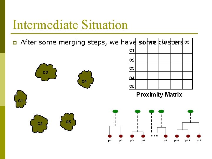
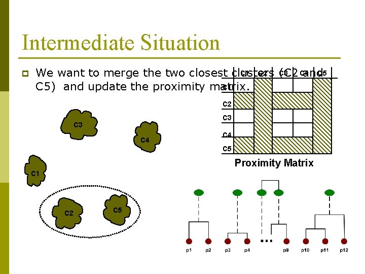
Intermediate Situation p C 1 C 2 clusters C 3 C 4 C 5 After some merging steps, we have some C 1 C 2 C 3 C 4 C 5 Proximity Matrix C 1 C 2 C 5

Intermediate Situation p C 1 C 2 C 3 C 4 C 5 We want to merge the two closest clusters (C 2 and C 1 C 5) and update the proximity matrix. C 2 C 3 C 4 C 5 Proximity Matrix C 1 C 2 C 5

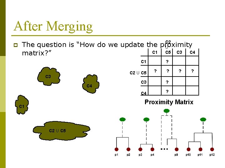
After Merging p C 2 The question is “How do we update the proximity U C 1 C 4 C 5 C 3 matrix? ” C 1 C 2 U C 5 C 3 C 4 ? ? ? C 3 ? C 4 ? ? ? Proximity Matrix C 1 C 2 U C 5

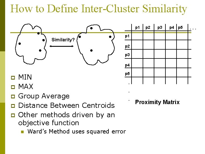
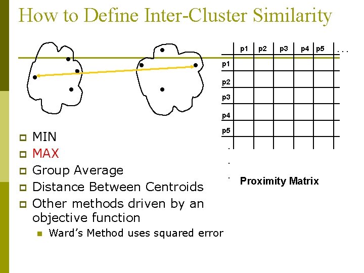
How to Define Inter-Cluster Similarity p 1 Similarity? p 2 p 3 p 4 p 5 p 1 p 2 p 3 p 4 p p p MIN MAX Group Average Distance Between Centroids Other methods driven by an objective function n p 5 Ward’s Method uses squared error . . . Proximity Matrix . . .

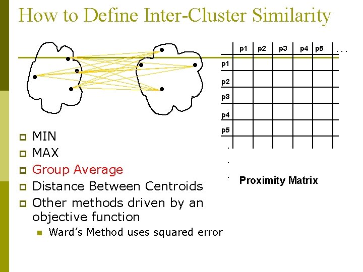
How to Define Inter-Cluster Similarity p 1 p 2 p 3 p 4 p 5 p 1 p 2 p 3 p 4 p p p MIN MAX Group Average Distance Between Centroids Other methods driven by an objective function n p 5 Ward’s Method uses squared error . . . Proximity Matrix . . .

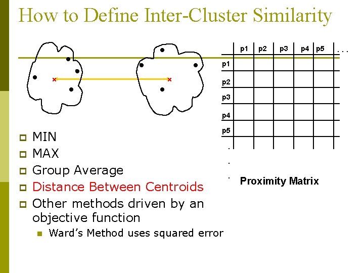
How to Define Inter-Cluster Similarity p 1 p 2 p 3 p 4 p 5 p 1 p 2 p 3 p 4 p p p MIN MAX Group Average Distance Between Centroids Other methods driven by an objective function n p 5 Ward’s Method uses squared error . . . Proximity Matrix . . .

How to Define Inter-Cluster Similarity p 1 p 2 p 3 p 4 p 5 p 1 p 2 p 3 p 4 p p p MIN MAX Group Average Distance Between Centroids Other methods driven by an objective function n p 5 Ward’s Method uses squared error . . . Proximity Matrix . . .

How to Define Inter-Cluster Similarity p 1 p 2 p 3 p 4 p 5 p 1 p 2 p 3 p 4 p p p MIN MAX Group Average Distance Between Centroids Other methods driven by an objective function n p 5 Ward’s Method uses squared error . . . Proximity Matrix . . .

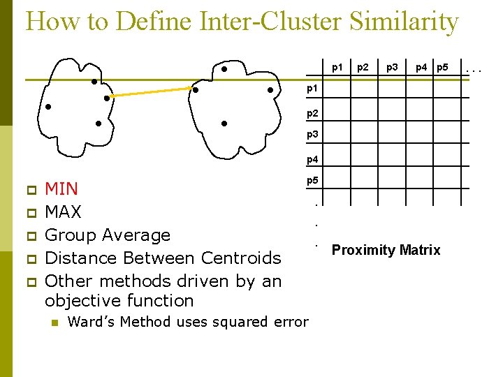
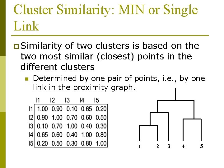
Cluster Similarity: MIN or Single Link p Similarity of two clusters is based on the two most similar (closest) points in the different clusters n Determined by one pair of points, i. e. , by one link in the proximity graph. 1 2 3 4 5

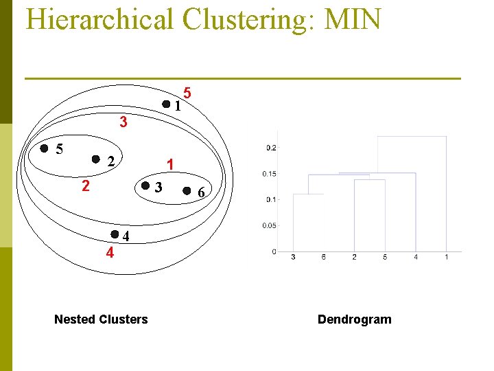
Hierarchical Clustering: MIN 1 3 5 2 1 2 3 4 5 6 4 Nested Clusters Dendrogram

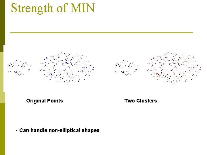
Strength of MIN Original Points • Can handle non-elliptical shapes Two Clusters

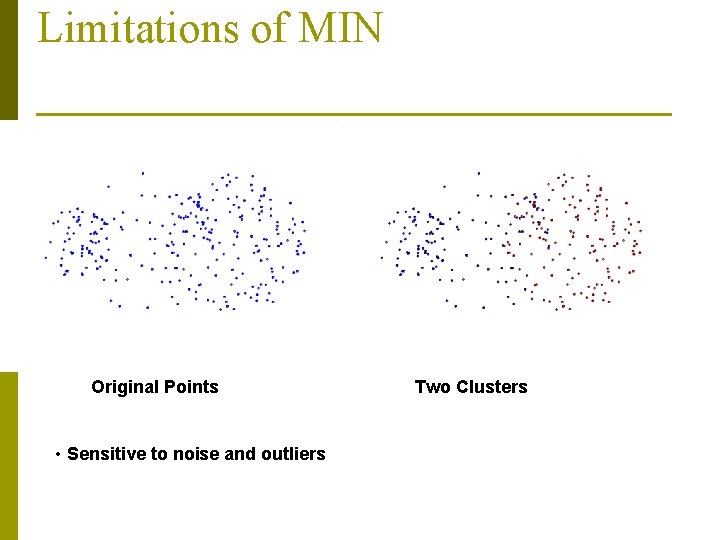
Limitations of MIN Original Points • Sensitive to noise and outliers Two Clusters

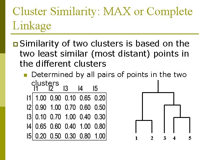
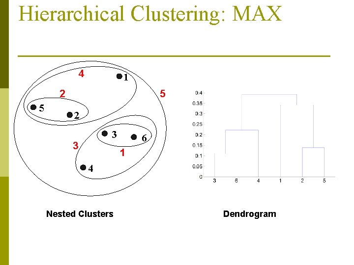
Cluster Similarity: MAX or Complete Linkage p Similarity of two clusters is based on the two least similar (most distant) points in the different clusters n Determined by all pairs of points in the two clusters 1 2 3 4 5

Hierarchical Clustering: MAX 4 1 2 5 5 2 3 3 6 1 4 Nested Clusters Dendrogram

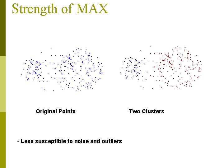
Strength of MAX Original Points • Less susceptible to noise and outliers Two Clusters

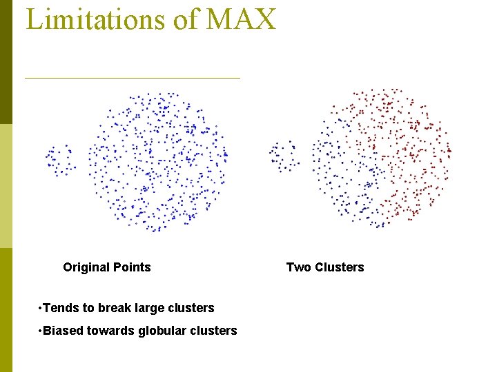
Limitations of MAX Original Points • Tends to break large clusters • Biased towards globular clusters Two Clusters

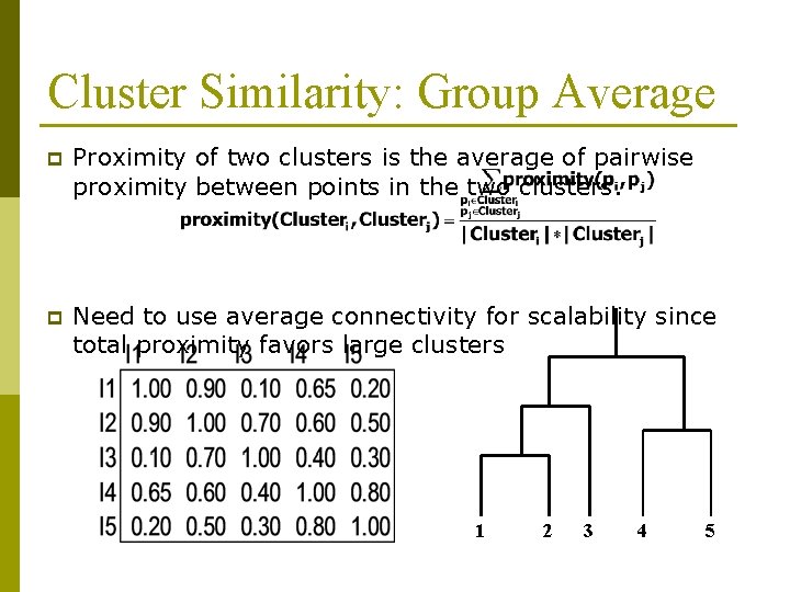
Cluster Similarity: Group Average p Proximity of two clusters is the average of pairwise proximity between points in the two clusters. p Need to use average connectivity for scalability since total proximity favors large clusters 1 2 3 4 5

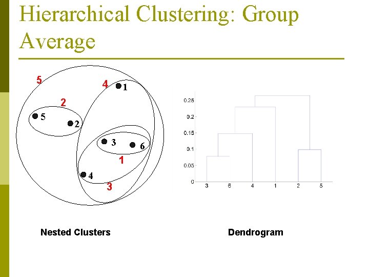
Hierarchical Clustering: Group Average 5 4 1 2 5 2 3 6 1 4 3 Nested Clusters Dendrogram

Hierarchical Clustering: Group Average p Compromise between Single and Complete Link p Strengths n p Less susceptible to noise and outliers Limitations n Biased towards globular clusters

Cluster Similarity: Ward’s Method p Similarity of two clusters is based on the increase in squared error when two clusters are merged n Similar to group average if distance between points is distance squared p Less susceptible to noise and outliers p Biased towards globular clusters p Hierarchical n analogue of K-means Can be used to initialize K-means

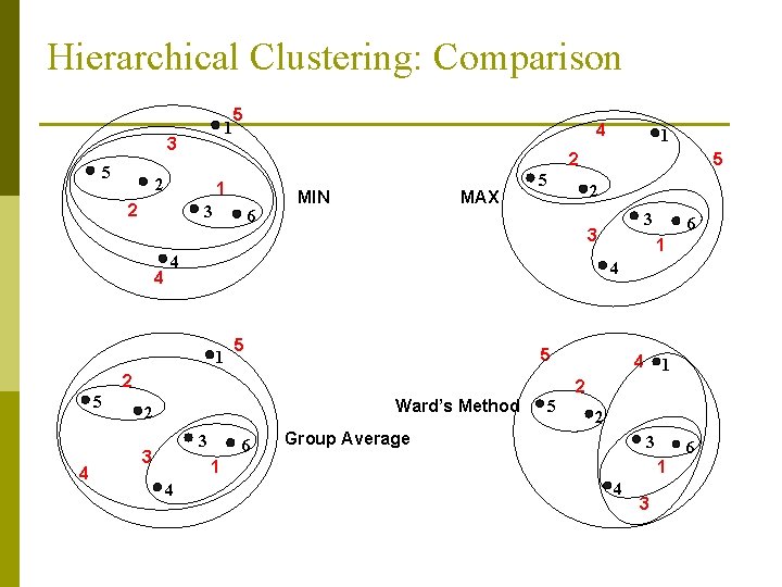
Hierarchical Clustering: Comparison 1 3 5 5 1 2 3 6 MIN MAX 5 2 5 1 5 Ward’s Method 3 6 4 1 2 5 2 Group Average 3 1 4 6 4 2 3 3 3 2 4 5 4 1 5 1 2 2 4 4 6 1 4 3

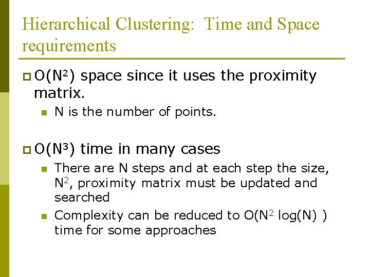
Hierarchical Clustering: Time and Space requirements p O(N 2) space since it uses the proximity matrix. n N is the number of points. p O(N 3) n n time in many cases There are N steps and at each step the size, N 2, proximity matrix must be updated and searched Complexity can be reduced to O(N 2 log(N) ) time for some approaches

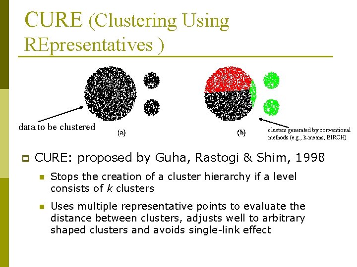
CURE (Clustering Using REpresentatives ) data to be clustered p clusters generated by conventional methods (e. g. , k-means, BIRCH) CURE: proposed by Guha, Rastogi & Shim, 1998 n Stops the creation of a cluster hierarchy if a level consists of k clusters n Uses multiple representative points to evaluate the distance between clusters, adjusts well to arbitrary shaped clusters and avoids single-link effect

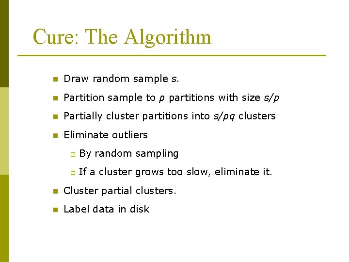
Cure: The Algorithm n Draw random sample s. n Partition sample to p partitions with size s/p n Partially cluster partitions into s/pq clusters n Eliminate outliers p By random sampling p If a cluster grows too slow, eliminate it. n Cluster partial clusters. n Label data in disk

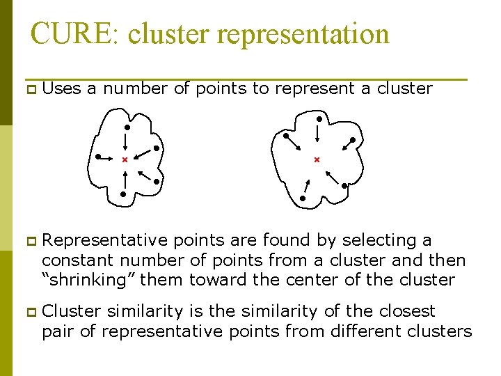
CURE: cluster representation p Uses a number of points to represent a cluster p Representative points are found by selecting a constant number of points from a cluster and then “shrinking” them toward the center of the cluster p Cluster similarity is the similarity of the closest pair of representative points from different clusters

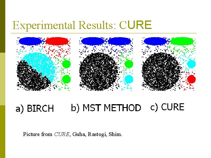
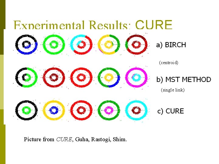
CURE p Shrinking representative points toward the center helps avoid problems with noise and outliers p CURE is better able to handle clusters of arbitrary shapes and sizes

Experimental Results: CURE Picture from CURE, Guha, Rastogi, Shim.

Experimental Results: CURE (centroid) (single link) Picture from CURE, Guha, Rastogi, Shim.

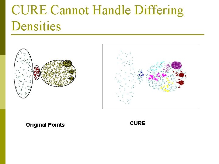
CURE Cannot Handle Differing Densities Original Points CURE

ROCK (RObust Clustering using lin. Ks) p Clustering algorithm for data with categorical and Boolean attributes n n 1. 2. 3. 4. A pair of points is defined to be neighbors if their similarity is greater than some threshold Use a hierarchical clustering scheme to cluster the data. Obtain a sample of points from the data set Compute the link value for each set of points, i. e. , transform the original similarities (computed by Jaccard coefficient) into similarities that reflect the number of shared neighbors between points Perform an agglomerative hierarchical clustering on the data using the “number of shared neighbors” as similarity measure and maximizing “the shared neighbors” objective function Assign the remaining points to the clusters that have been found

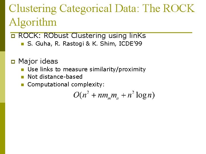
Clustering Categorical Data: The ROCK Algorithm p ROCK: RObust Clustering using lin. Ks n p S. Guha, R. Rastogi & K. Shim, ICDE’ 99 Major ideas n n n Use links to measure similarity/proximity Not distance-based Computational complexity:

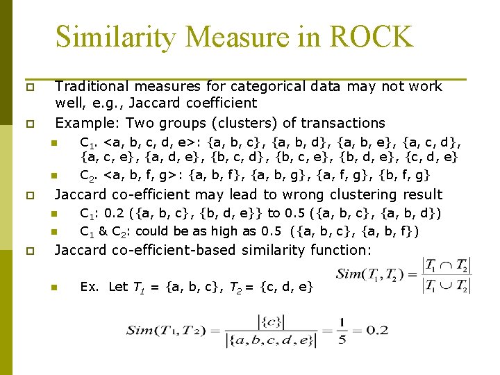
Similarity Measure in ROCK p p Traditional measures for categorical data may not work well, e. g. , Jaccard coefficient Example: Two groups (clusters) of transactions n n p Jaccard co-efficient may lead to wrong clustering result n n p C 1. <a, b, c, d, e>: {a, b, c}, {a, b, d}, {a, b, e}, {a, c, d}, {a, c, e}, {a, d, e}, {b, c, d}, {b, c, e}, {b, d, e}, {c, d, e} C 2. <a, b, f, g>: {a, b, f}, {a, b, g}, {a, f, g}, {b, f, g} C 1: 0. 2 ({a, b, c}, {b, d, e}} to 0. 5 ({a, b, c}, {a, b, d}) C 1 & C 2: could be as high as 0. 5 ({a, b, c}, {a, b, f}) Jaccard co-efficient-based similarity function: n Ex. Let T 1 = {a, b, c}, T 2 = {c, d, e}

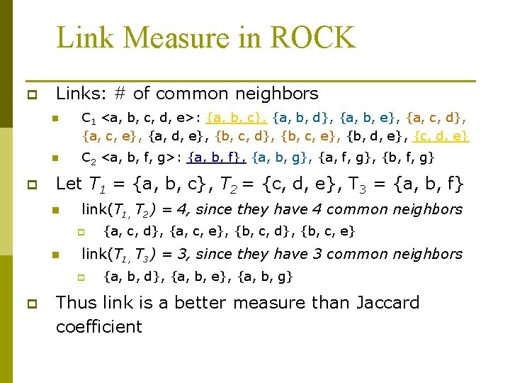
Link Measure in ROCK p p Links: # of common neighbors n C 1 <a, b, c, d, e>: {a, b, c}, {a, b, d}, {a, b, e}, {a, c, d}, {a, c, e}, {a, d, e}, {b, c, d}, {b, c, e}, {b, d, e}, {c, d, e} n C 2 <a, b, f, g>: {a, b, f}, {a, b, g}, {a, f, g}, {b, f, g} Let T 1 = {a, b, c}, T 2 = {c, d, e}, T 3 = {a, b, f} n link(T 1, T 2) = 4, since they have 4 common neighbors p n link(T 1, T 3) = 3, since they have 3 common neighbors p p {a, c, d}, {a, c, e}, {b, c, d}, {b, c, e} {a, b, d}, {a, b, e}, {a, b, g} Thus link is a better measure than Jaccard coefficient

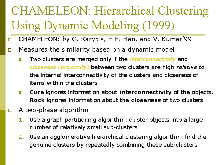
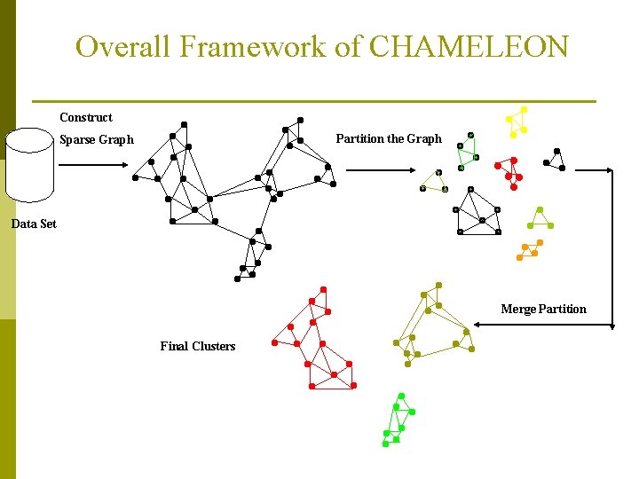
CHAMELEON: Hierarchical Clustering Using Dynamic Modeling (1999) p CHAMELEON: by G. Karypis, E. H. Han, and V. Kumar’ 99 p Measures the similarity based on a dynamic model p n Two clusters are merged only if the interconnectivity and closeness (proximity) between two clusters are high relative to the internal interconnectivity of the clusters and closeness of items within the clusters n Cure ignores information about interconnectivity of the objects, Rock ignores information about the closeness of two clusters A two-phase algorithm 1. Use a graph partitioning algorithm: cluster objects into a large number of relatively small sub-clusters 2. Use an agglomerative hierarchical clustering algorithm: find the genuine clusters by repeatedly combining these sub-clusters

Overall Framework of CHAMELEON Construct Partition the Graph Sparse Graph Data Set Merge Partition Final Clusters

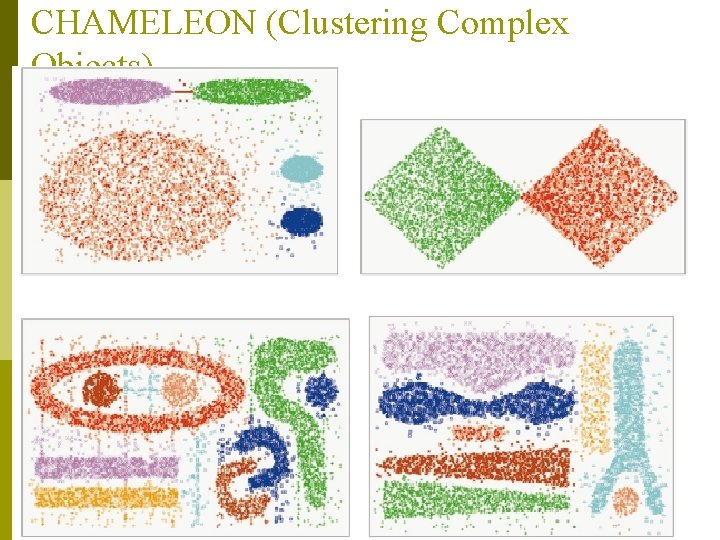
CHAMELEON (Clustering Complex Objects)

Cluster Analysis p What is Cluster Analysis? p Types of Data in Cluster Analysis p A Categorization of Major Clustering Methods p Partitioning Methods p Hierarchical Methods p Density-Based Methods p Grid-Based Methods p Model-Based Clustering Methods p Outlier Analysis p Summary

Density-Based Clustering Methods p p Clustering based on density (local cluster criterion), such as density-connected points Major features: n n p Discover clusters of arbitrary shape Handle noise One scan Need density parameters as termination condition Several interesting studies: n n DBSCAN: Ester, et al. (KDD’ 96) OPTICS: Ankerst, et al (SIGMOD’ 99). DENCLUE: Hinneburg & D. Keim (KDD’ 98) CLIQUE: Agrawal, et al. (SIGMOD’ 98)

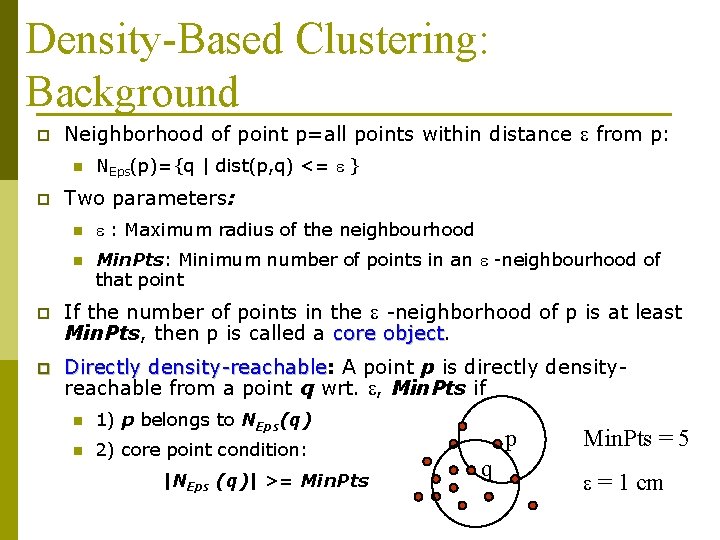
Density-Based Clustering: Background p Neighborhood of point p=all points within distance e from p: n p NEps(p)={q | dist(p, q) <= e } Two parameters: n e : Maximum radius of the neighbourhood n Min. Pts: Minimum number of points in an e -neighbourhood of that point p If the number of points in the e -neighborhood of p is at least Min. Pts, then p is called a core object p Directly density-reachable: density-reachable A point p is directly densityreachable from a point q wrt. e, Min. Pts if n 1) p belongs to NEps(q) n 2) core point condition: |NEps (q)| >= Min. Pts p q Min. Pts = 5 e = 1 cm

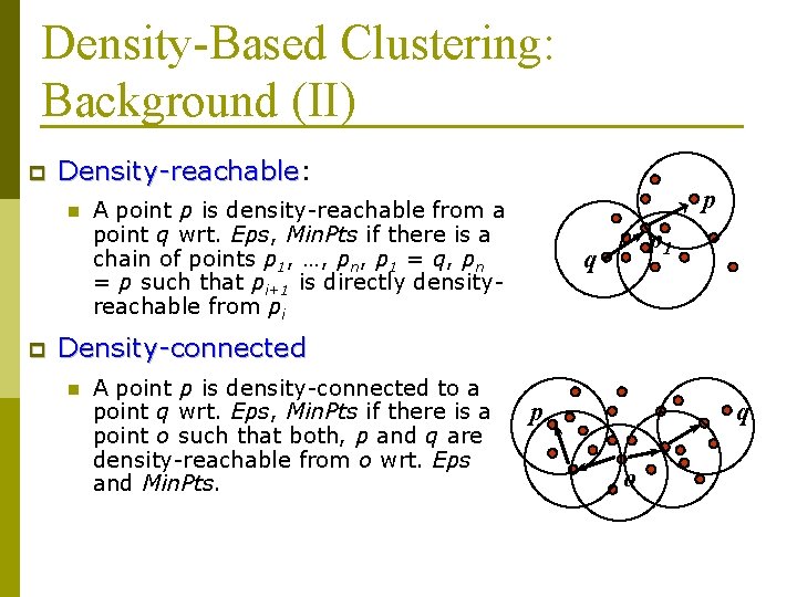
Density-Based Clustering: Background (II) p Density-reachable: Density-reachable n p p A point p is density-reachable from a point q wrt. Eps, Min. Pts if there is a chain of points p 1, …, pn, p 1 = q, pn = p such that pi+1 is directly densityreachable from pi p 1 q Density-connected n A point p is density-connected to a point q wrt. Eps, Min. Pts if there is a point o such that both, p and q are density-reachable from o wrt. Eps and Min. Pts. p q o

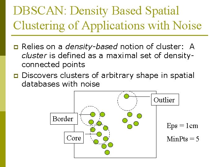
DBSCAN: Density Based Spatial Clustering of Applications with Noise p p Relies on a density-based notion of cluster: A cluster is defined as a maximal set of densityconnected points Discovers clusters of arbitrary shape in spatial databases with noise Outlier Border Core Eps = 1 cm Min. Pts = 5

DBSCAN: The Algorithm n Arbitrary select a point p n Retrieve all points density-reachable from p wrt Eps and Min. Pts. n If p is a core point, a cluster is formed. n If p is a border point, no points are density-reachable from p and DBSCAN visits the next point of the database. n Continue the process until all of the points have been processed.