Cluster Analysis First used by Tryon 1939 encompasses

Cluster Analysis

First used by Tryon (1939) encompasses a number of different algorithms and methods for grouping objects of similar kind into respective categories. 2

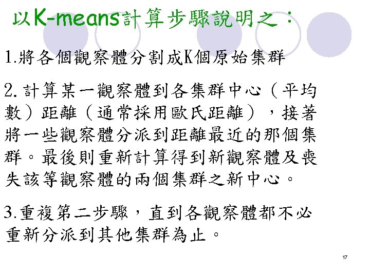
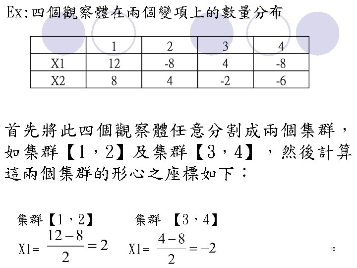
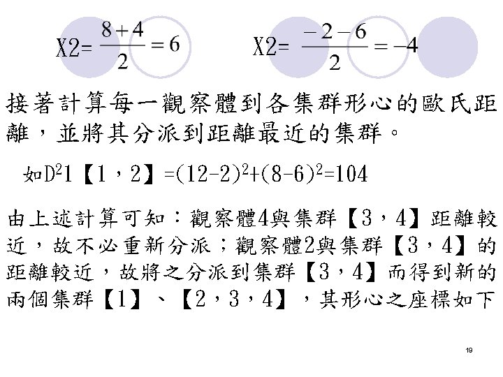
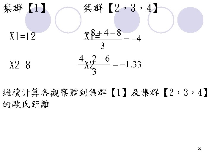
Two-stage Cluster Sampling When Clusters are of Unequal Size l l l Desired Sample Proportion p=n/N a: Desired # of Clusters Selected in the 1 st Stage A: Total # of Clusters b: Sample Size within Each Cluster Selected Ni : # of Elements in Cluster i 22

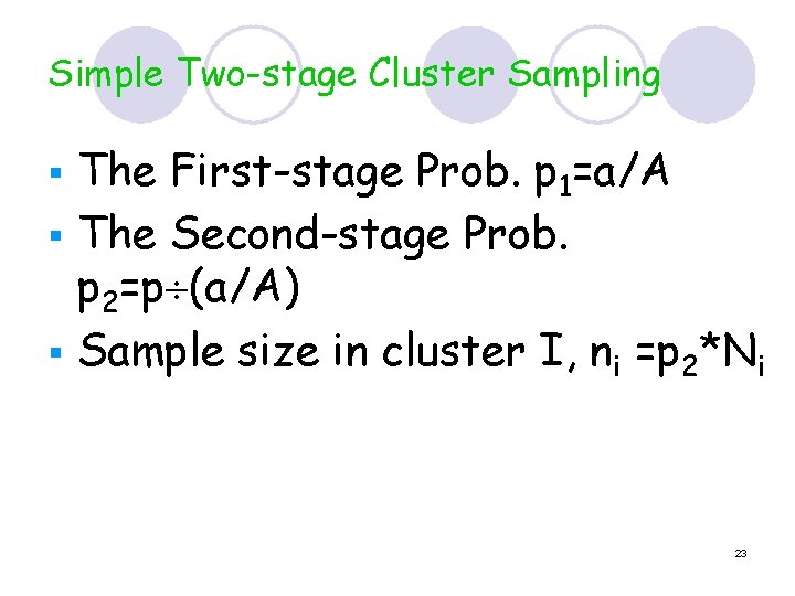
Simple Two-stage Cluster Sampling The First-stage Prob. p 1=a/A § The Second-stage Prob. p 2=p (a/A) § Sample size in cluster I, ni =p 2*Ni § 23

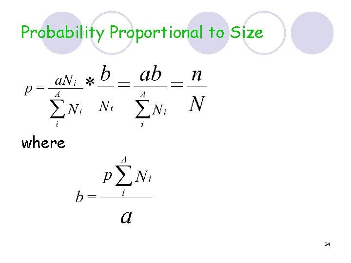
Probability Proportional to Size where 24

Example l l Draw a sample of 1, 000 households from a city that contains about 200, 000 households distributed among 2000 blocks of unequal but known size. The desired sample proportion =1/200 The desired # of clusters selected in the 1 st stage=100 How do we conduct the two-stage cluster sampling? 25

What is Cluster Analysis? n n Cluster Analysis is a class of statistical techniques that can be applied to data that exhibit natural groupings. CA is an interdependence technique that makes no distinction between dependent and independent variables. There is NO statistical significance testing in CA. CA is more a group of different algorithms that put objects into clusters following “well-defined similarity rules. ” 26

What is A Cluster? l. A cluster is a group of relatively homogeneous cases and observations. l Clusters exhibit high internal homogeneity and high external heterogeneity. 27

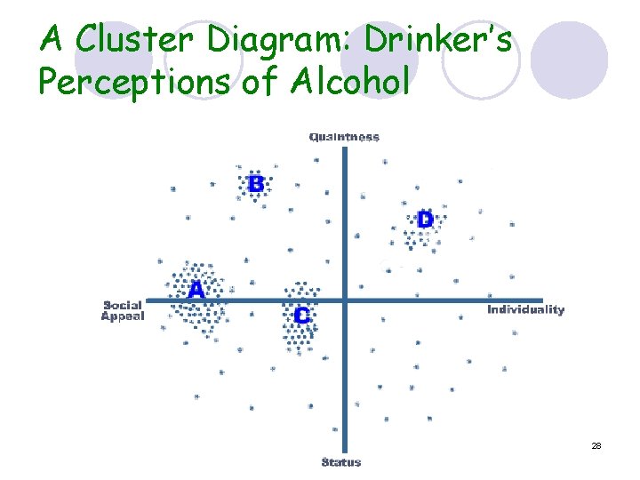
A Cluster Diagram: Drinker’s Perceptions of Alcohol 28

Characteristics of CA Cluster Analysis is a tool of discovery. l It discovers structures in data but does NOT explain why they exist. l CA is used when we do not have an a priori hypothesis, but when we are in the exploratory phase. l 29

How does CA differ… l From Discriminant Analysis ¡A dependence technique ¡Predict the probability that an object will fall into one of two or more mutually exclusive categories based on several independent variables. ¡Find a linear combination of independent variables. ¡Find natural groupings based on distances among objects. 30

l From Factor Analysis ¡Similar to cluster analysis in that it is an interdependence technique. ¡Primary difference lies in the focus on objects and variables. ¡Factor analysis reduces variables to a few factors. Cluster analysis reduces objects to a few clusters. 31

Cluster Analysis Methods l Three Cluster Analysis Methods ¡Joining (Tree Clustering) ¡Two-way Joining ¡K-means Testing 32

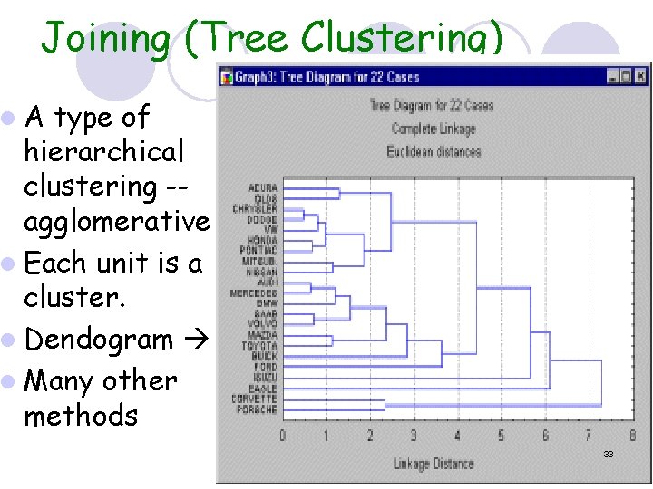
Joining (Tree Clustering) l. A type of hierarchical clustering -agglomerative l Each unit is a cluster. l Dendogram l Many other methods 33

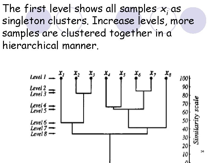
The first level shows all samples xi as singleton clusters. Increase levels, more samples are clustered together in a hierarchical manner. 34

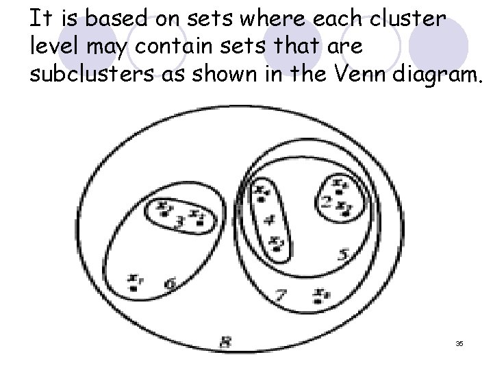
It is based on sets where each cluster level may contain sets that are subclusters as shown in the Venn diagram. 35

Two-way Joining Hartigan (1975) l Two-way Joining tries to cluster both variables and objects. l Only useful if you think clustering along BOTH lines will be useful. l Very rare in application. 36

k-Means Clustering: Begin with a preconception about the number of clusters (k). l Thought of as ANOVA in reverse. l ANOVA evaluates between group var. against within group var. when computing stat. signif. of hypothesis that groups are different. l In k-Means the computer will try to move objects in and out of the groups to get the most significant ANOVA results. l 37

It’s all about distance… l Distance Measures ¡Euclidean Distance ¡Squared Euclidean Distance ¡Manhattan Distance ¡Chebychev Distance ¡Power Distance 38

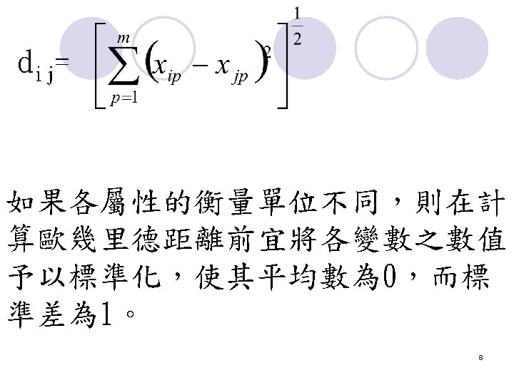
EQUATION: Euclidean Distance l Basic equation for determining distance measure. l Distance (x, y) = {Σi (xi – yi)2}1/2 l A standard formula for determining the distance between two points on a plane 39

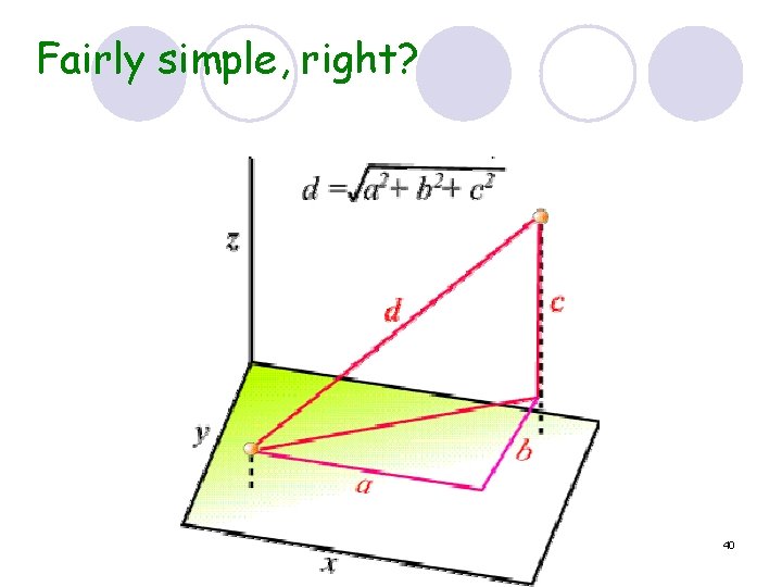
Fairly simple, right? 40

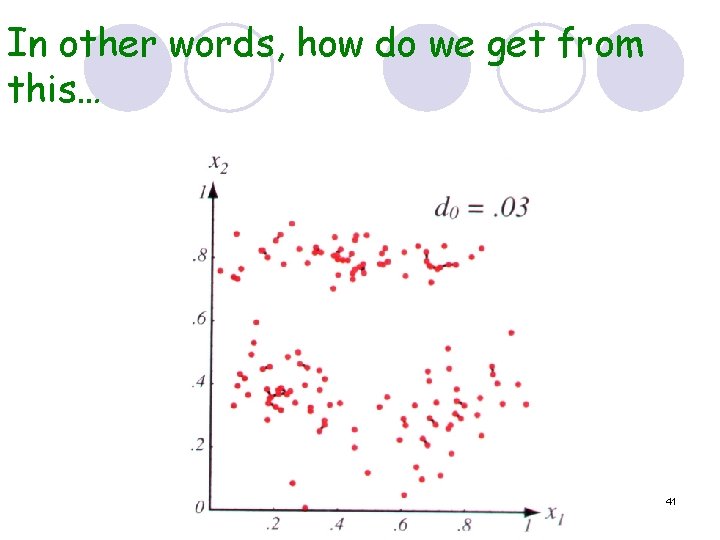
In other words, how do we get from this… 41

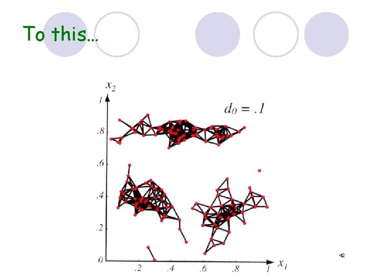
To this… 42

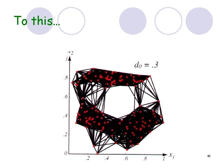
To this… 43

How to Determine Clusters. l Use a computer. l Call a professional. 44

Clusters in the Real World 45

Why is Cluster Analysis Important? l Relatively new/evolving technique l Highly useful for market segmentation l Segmentation = identifying groupings of customers using statistical multi-variate analysis, often based on perceptions and attitudes as well as demographics and behavior. l Segmentation helpful to small companies attempting to carve out a niche l Large companies trying to tailor their products/services to different segments 46

In addition to segmentation, clusters are used to… l Design products and establish brands l Target direct mail l Make decisions about customer conversion and retention l Decide on marketing cost levels 47

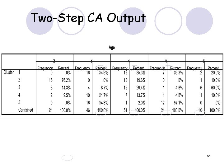
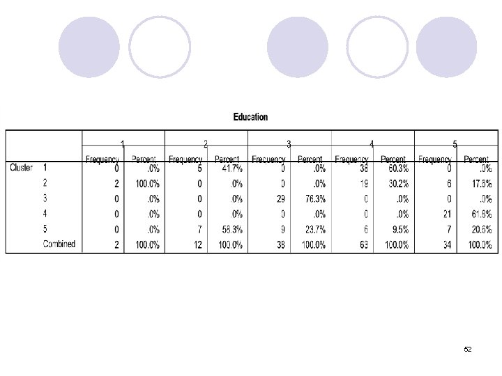
Ex: Luxury Car Customers l Demographic examples easier to illustrate l Demographics: ¡Gender ¡Education ¡Age l 149 customers (objects) of a luxury car dealership 48

Using SPSS for Clustering l Chose “Two. Step Cluster Analysis” ¡ Basically, the agglomerative technique (dendogram). ¡ Step One: Creates very small (individual) sub-clusters. ¡ Step Two: Cluster sub-clusters into desired number of clusters. ¡ Automatically finds optimum number of clusters. 49

Two-Step CA Output What are these clusters? 50

Two-Step CA Output 51

52

53

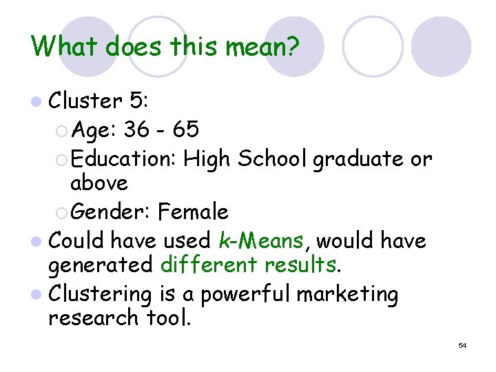
What does this mean? l Cluster 5: ¡ Age: 36 - 65 ¡ Education: High School graduate or above ¡ Gender: Female l Could have used k-Means, would have generated different results. l Clustering is a powerful marketing research tool. 54

Claritas: Clustering Experts l Example: Claritas Corporation ¡ Claritas founded the U. S. geodemographic industry when it launched the first PRIZM segmentation system in 1974. ¡ PRIZM (Potential Rating Index for Zip Markets) categorizes every U. S. neighborhood into 1 of 62 “clusters. ” ¡ Descriptive Names: l Money and Brains l Young Literati l Shotguns and Pickups 55

Money and Brains l Sophisticated Urban Fringe Couples ¡ Cluster is a mix of family types: singles, married couples with children and married couples without children. These families own their homes in upscale neighborhoods near cities. Dual incomes provide luxuries, travel and entertainment. ¡ Demographics: l Affluent l Age Groups: 55 -64, 65+ l Predominantly White, High Asian 56

Clusters Work! l At a conservative estimate, more than 20, 000 companies in the United States and Canada alone used clusters as part of their marketing information mix last year. 57

Web Sources l l l l l http: //cwis. livjm. ac. uk/busrmccl/ae 230/lect 10. ppt http: //www. clusterbigip 1. claritas. com/claritas/Default. jsp? main=3&su bmenu=seg&subcat=segprizmne http: //www. insightsc. ie/newsletter 7. htm http: //www. directionsmag. com/article. asp? article_id=12 http: //fun. supereva. it/scoleri. freeweb/cern/biografie/hawking. jpg http: //www. statsoft. com/textbook/stcluan. html http: //www-db. stanford. edu/~ullman/mining/cluster 1. pdf http: //www. snr. missouri. edu/multivariate/Cluster. Analysis. pdf 58

Print Sources Recent Developments in Clustering and Data Analysis. Edited by Chikio Hayashi, Edwin Diday, Michel Jambou, Noboru Ohsumi. Academic Press, Inc. 1988. l Finding Groups in Data: An Introduction to Cluster Analysis. Leonard Kaufman, Peter J. Rousseeuw. John Wiley and Sons, Inc. 1990. l Marketing Research: An Aid to Decision Making. Dr. Alan T. Shao. South-Western. 2002. l Exploring Marketing Research. William G. Zikmund. South-Western. 2003. l 59

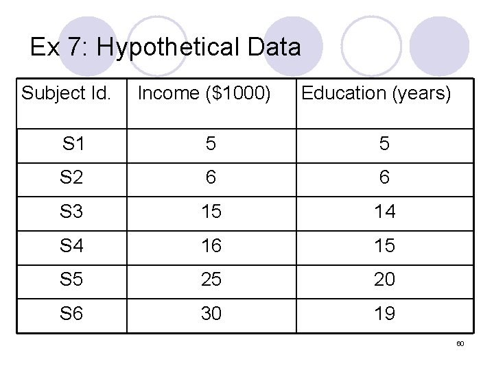
Ex 7: Hypothetical Data Subject Id. Income ($1000) Education (years) S 1 5 5 S 2 6 6 S 3 15 14 S 4 16 15 S 5 25 20 S 6 30 19 60

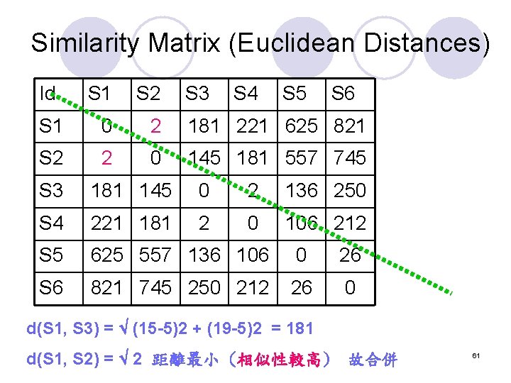
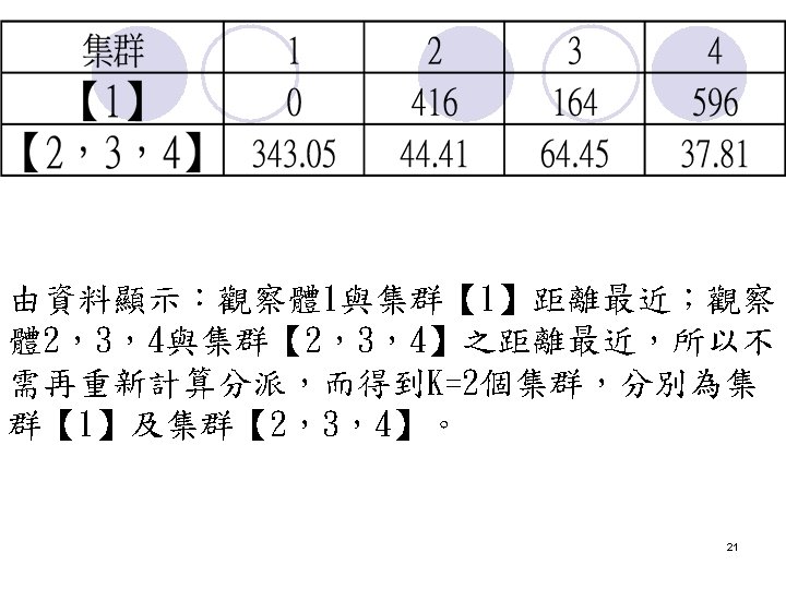
Similarity Matrix (Euclidean Distances) Id S 1 S 2 S 3 S 4 S 5 S 6 S 1 0 2 181 221 625 821 S 2 2 0 145 181 557 745 S 3 181 145 0 2 136 250 S 4 221 181 2 0 106 212 S 5 625 557 136 106 0 26 S 6 821 745 250 212 26 0 d(S 1, S 3) = (15 -5)2 + (19 -5)2 = 181 d(S 1, S 2) = 2 距離最小 (相似性較高) 故合併 61

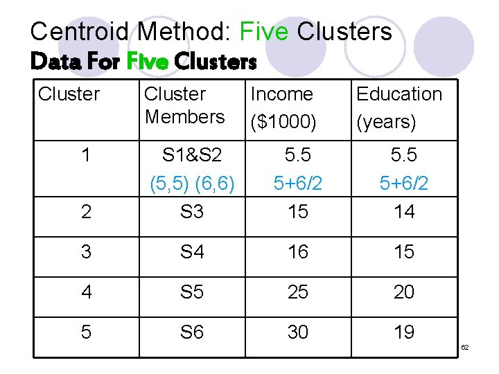
Centroid Method: Five Clusters Data For Five Clusters Cluster 1 Cluster Members Income ($1000) Education (years) 2 S 1&S 2 (5, 5) (6, 6) S 3 5. 5 5+6/2 15 5. 5 5+6/2 14 3 S 4 16 15 4 S 5 25 20 5 S 6 30 19 62

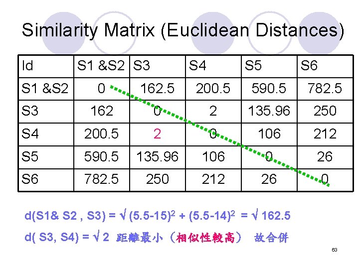
Similarity Matrix (Euclidean Distances) Id S 1 &S 2 S 3 S 4 S 5 S 6 0 162. 5 200. 5 590. 5 782. 5 S 3 162 0 2 135. 96 250 S 4 200. 5 2 0 106 212 S 5 590. 5 135. 96 106 0 26 S 6 782. 5 250 212 26 0 d(S 1& S 2 , S 3) = (5. 5 -15)2 + (5. 5 -14)2 = 162. 5 d( S 3, S 4) = 2 距離最小 (相似性較高) 故合併 63

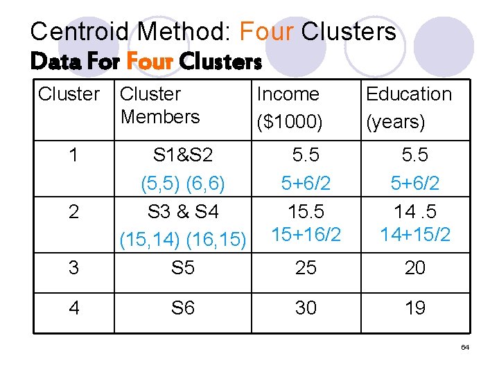
Centroid Method: Four Clusters Data For Four Clusters Cluster 1 Cluster Members Income ($1000) Education (years) 5. 5 5+6/2 15. 5 15+16/2 5. 5 5+6/2 14. 5 14+15/2 3 S 1&S 2 (5, 5) (6, 6) S 3 & S 4 (15, 14) (16, 15) S 5 25 20 4 S 6 30 19 2 64

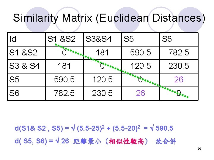
Similarity Matrix (Euclidean Distances) Id S 1 &S 2 S 3&S 4 S 5 S 6 S 1 &S 2 0 181 590. 5 782. 5 S 3 & S 4 181 0 120. 5 230. 5 S 5 590. 5 120. 5 0 26 S 6 782. 5 230. 5 26 0 d(S 1& S 2 , S 5) = (5. 5 -25)2 + (5. 5 -20)2 = 590. 5 d( S 5, S 6) = 26 距離最小 (相似性較高) 故合併 65

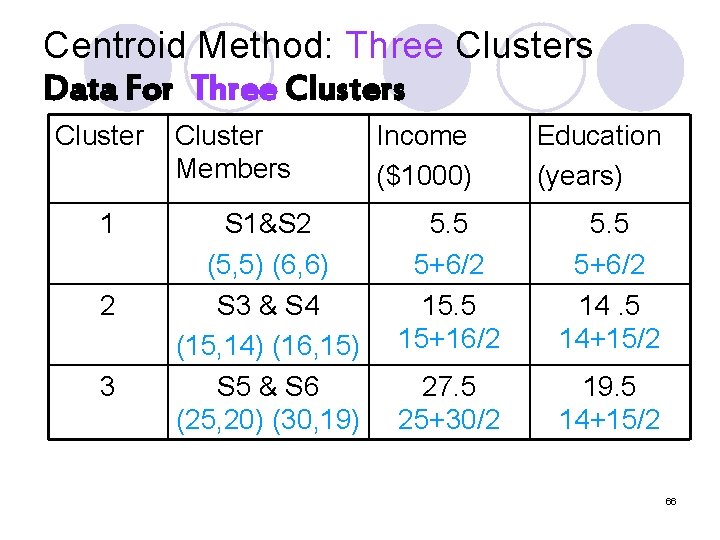
Centroid Method: Three Clusters Data For Three Clusters Cluster 1 2 3 Cluster Members S 1&S 2 (5, 5) (6, 6) S 3 & S 4 (15, 14) (16, 15) S 5 & S 6 (25, 20) (30, 19) Income ($1000) Education (years) 5. 5 5+6/2 15. 5 15+16/2 5. 5 5+6/2 14. 5 14+15/2 27. 5 25+30/2 19. 5 14+15/2 66

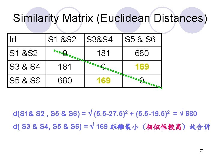
Similarity Matrix (Euclidean Distances) Id S 1 &S 2 S 3&S 4 S 5 & S 6 S 1 &S 2 0 181 680 S 3 & S 4 181 0 169 S 5 & S 6 680 169 0 d(S 1& S 2 , S 5 & S 6) = (5. 5 -27. 5)2 + (5. 5 -19. 5)2 = 680 d( S 3 & S 4, S 5 & S 6) = 169 距離最小 (相似性較高) 故合併 67

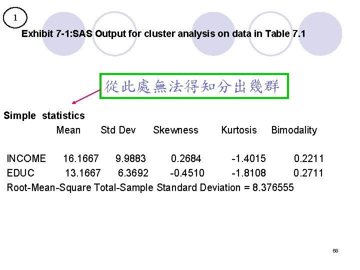
1 Exhibit 7 -1: SAS Output for cluster analysis on data in Table 7. 1 從此處無法得知分出幾群 Simple statistics Mean Std Dev Skewness Kurtosis Bimodality INCOME 16. 1667 9. 9883 0. 2684 -1. 4015 0. 2211 EDUC 13. 1667 6. 3692 -0. 4510 -1. 8108 0. 2711 Root-Mean-Square Total-Sample Standard Deviation = 8. 376555 68

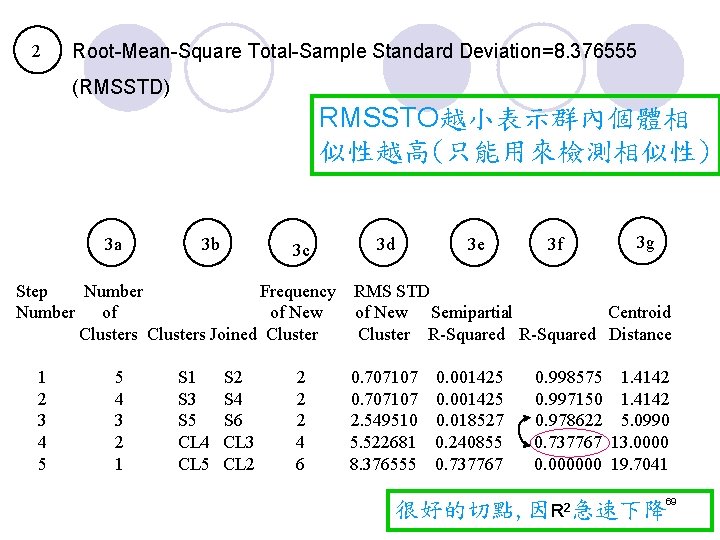
2 Root-Mean-Square Total-Sample Standard Deviation=8. 376555 (RMSSTD) RMSSTO越小表示群內個體相 似性越高(只能用來檢測相似性) 3 a 3 b 3 c Step Number Frequency Number of of New Clusters Joined Cluster 1 2 3 4 5 5 4 3 2 1 S 3 S 5 CL 4 CL 5 S 2 S 4 S 6 CL 3 CL 2 2 4 6 3 d 3 e 3 f 3 g RMS STD of New Semipartial Centroid Cluster R-Squared Distance 0. 707107 0. 001425 2. 549510 0. 018527 5. 522681 0. 240855 8. 376555 0. 737767 0. 998575 1. 4142 0. 997150 1. 4142 0. 978622 5. 0990 0. 737767 13. 0000 0. 000000 19. 7041 很好的切點, 因R 2急速下降69

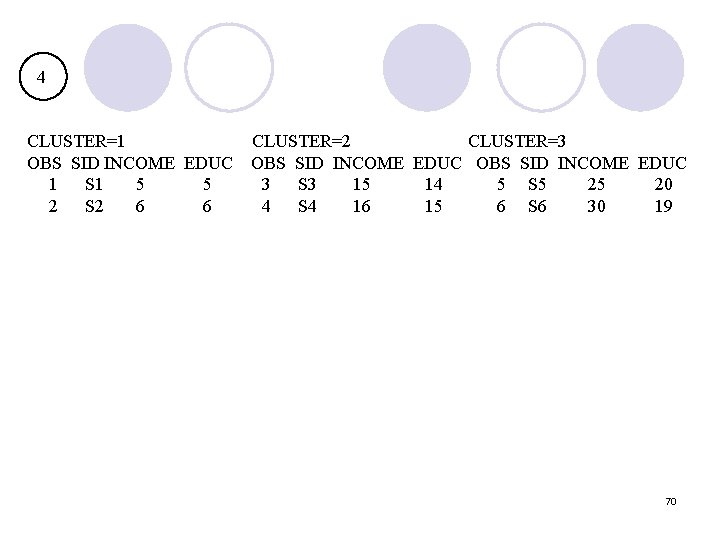
4 CLUSTER=1 OBS SID INCOME EDUC 1 S 1 5 5 2 S 2 6 6 CLUSTER=2 CLUSTER=3 OBS SID INCOME EDUC 3 S 3 15 14 5 S 5 25 20 4 S 4 16 15 6 S 6 30 19 70

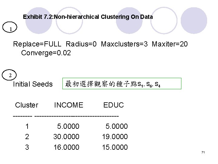
Exhibit 7. 2: Non-hierarchical Clustering On Data 1 Replace=FULL Radius=0 Maxclusters=3 Maxiter=20 Converge=0. 02 2 Initial Seeds 最初選擇觀察的種子點S 1, S 6, S 4 Cluster INCOME EDUC ---------------------1 5. 0000 2 30. 0000 19. 0000 3 16. 0000 15. 0000 71

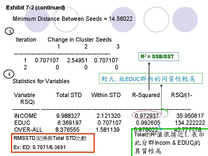
Exhibit 7 -2 (continued) Minimum Distance Between Seeds = 14. 56022 3 Iteration Change in Cluster Seeds 1 2 3 -------------------------1 0. 707107 2. 54951 0. 707107 2 0 0 0 4 Statistics for Variables R 2 = SSB/SST 較大. 故EDUC群內的同質性較高 Variable Total STD Within STD R-Squared RSQ/(1 RSQ) ----------------------------------------------INCOME 9. 988327 2. 121320 0. 972937 35. 950617 EDUC 6. 369197 0. 707107 0. 992605 134. 222222 OVER-ALL 8. 376555 1. 581139 0. 978622 45. 777778 RMSSTD: 記得與Total STD比較 Ex: ED: 0. 7071/6. 3691 Total的R 2值很接近 1. 表示 此分群Incom & EDUC 72的 異質性高

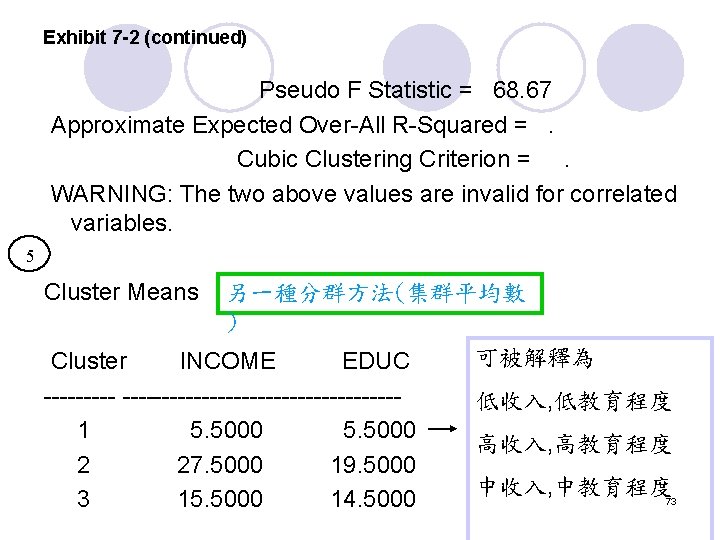
Exhibit 7 -2 (continued) Pseudo F Statistic = 68. 67 Approximate Expected Over-All R-Squared =. Cubic Clustering Criterion =. WARNING: The two above values are invalid for correlated variables. 5 Cluster Means 另一種分群方法(集群平均數 ) 可被解釋為 INCOME EDUC Cluster ----------------------1 5. 5000 2 27. 5000 19. 5000 3 15. 5000 14. 5000 低收入, 低教育程度 高收入, 高教育程度 中收入, 中教育程度 73

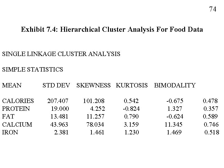
74 Exhibit 7. 4: Hierarchical Cluster Analysis For Food Data SINGLE LINKAGE CLUSTER ANALYSIS SIMPLE STATISTICS MEAN CALORIES PROTEIN FAT CALCIUM IRON STD DEV 207. 407 19. 000 13. 481 43. 963 2. 381 SKEWNESS KURTOSIS 101. 208 4. 252 11. 257 78. 034 1. 461 0. 542 -0. 824 0. 790 3. 159 1. 230 BIMODALITY -0. 675 1. 327 -0. 624 11. 345 1. 469 0. 478 0. 357 0. 589 0. 746 0. 518

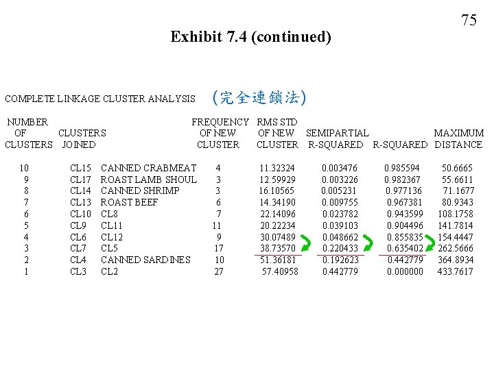
75 Exhibit 7. 4 (continued) COMPLETE LINKAGE CLUSTER ANALYSIS NUMBER OF CLUSTERS JOINED 10 9 8 7 6 5 4 3 2 1 CL 15 CL 17 CL 14 CL 13 CL 10 CL 9 CL 6 CL 7 CL 4 CL 3 (完全連鎖法) FREQUENCY RMS STD OF NEW SEMIPARTIAL MAXIMUM CLUSTER R-SQUARED DISTANCE CANNED CRABMEAT ROAST LAMB SHOUL CANNED SHRIMP ROAST BEEF CL 8 CL 11 CL 12 CL 5 CANNED SARDINES CL 2 4 3 3 6 7 11 9 17 10 27 11. 32324 12. 59929 16. 10565 14. 34190 22. 14096 20. 22234 30. 07489 38. 73570 51. 36181 57. 40958 0. 003476 0. 003226 0. 005231 0. 009755 0. 023782 0. 039103 0. 048662 0. 220433 0. 192623 0. 442779 0. 985594 0. 982367 0. 977136 0. 967381 0. 943599 0. 904496 0. 855835 0. 635402 0. 442779 0. 000000 50. 6665 55. 6611 71. 1677 80. 9343 108. 1758 141. 7814 154. 4447 262. 5666 364. 8934 433. 7617

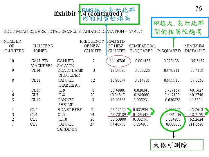
76 RMS越小表示此群 Exhibit 7. 4 (continued) 內的同質性越高 R 2越大. 表示此群 ROOT-MEAN-SQUARE TOTAL-SAMPLE STANDARD DEVIATION = 57. 4096 NUMBER OF CLUSTERS 10 CLUSTERS JOINED 9 CANNED MACKEREL CL 14 8 CL 11 7 6 5 CL 15 CL 7 CL 12 4 3 2 1 CL 6 CL 4 CL 3 CL 2 間的相異性越高 FREQUENCY RMS STD OF NEW SEMIPARTIAL MINIMUM CLUSTER R-SQUARED DISTANCE CANNED SALMON ROAST LAMB SHOULDER CANNED CRABMEAT CL 9 CL 8 CANNED SHRIMP ROAST BEEF CL 5 CL 10 CANNED SARDINES 2 11. 16786 0. 001455 0. 973438 35. 3159 3 12. 59929 0. 003226 0. 970211 35. 4131 12 16. 80697 0. 014701 0. 955510 39. 5267 8 20 3 20. 48901 40. 04817 16. 10565 0. 028341 0. 285060 0. 005231 0. 927169 0. 642109 0. 636878 40. 1627 40. 2746 44. 8504 21 24 26 27 43. 49500 48. 72189 50. 53988 57. 40958 0. 085924 0. 189548 0. 106595 0. 254811 0. 550954 0. 361406 0. 254811 0. 000000 45. 7642 48. 7139 62. 2624 211. 5691 太低可刪除

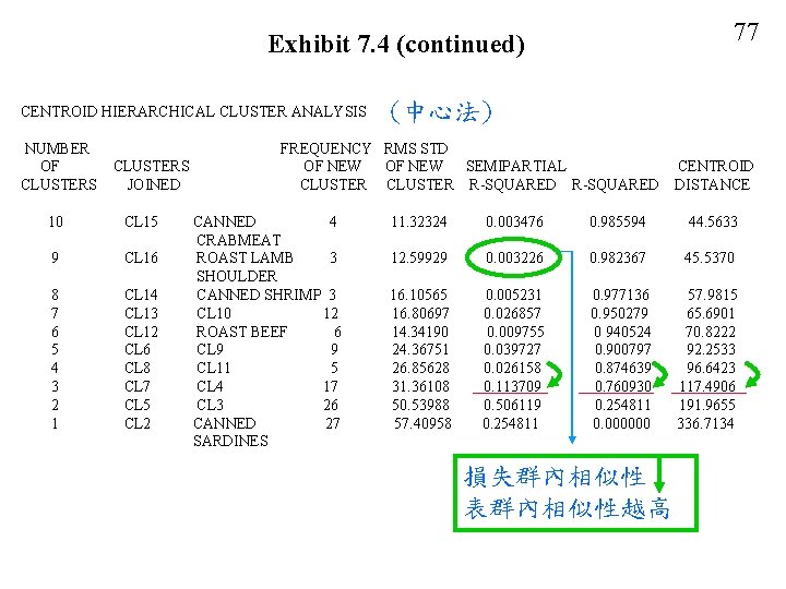
77 Exhibit 7. 4 (continued) CENTROID HIERARCHICAL CLUSTER ANALYSIS NUMBER OF CLUSTERS JOINED 10 CL 15 9 CL 16 8 7 6 5 4 3 2 1 CL 14 CL 13 CL 12 CL 6 CL 8 CL 7 CL 5 CL 2 (中心法) FREQUENCY RMS STD OF NEW SEMIPARTIAL CLUSTER R-SQUARED CANNED 4 CRABMEAT ROAST LAMB 3 SHOULDER CANNED SHRIMP 3 CL 10 12 ROAST BEEF 6 CL 9 9 CL 11 5 CL 4 17 CL 3 26 CANNED 27 SARDINES CENTROID DISTANCE 11. 32324 0. 003476 0. 985594 44. 5633 12. 59929 0. 003226 0. 982367 45. 5370 16. 10565 16. 80697 14. 34190 24. 36751 26. 85628 31. 36108 50. 53988 57. 40958 0. 005231 0. 026857 0. 009755 0. 039727 0. 026158 0. 113709 0. 506119 0. 254811 0. 977136 0. 950279 0 940524 0. 900797 0. 874639 0. 760930 0. 254811 0. 000000 57. 9815 65. 6901 70. 8222 92. 2533 96. 6423 117. 4906 191. 9655 336. 7134 損失群內相似性 表群內相似性越高

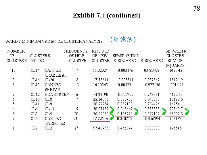
Exhibit 7. 4 (continued) WARD'S MINIMUM VARIANCE CLUSTER ANALYSIS NUMBER OF CLUSTERS JOINED 10 CL 14 9 8 CL 16 CL 15 7 6 5 4 3 2 CL 10 CL 11 CL 6 CL 5 CL 3 1 CL 7 (華德法) FREQUENCY RMS STD BETWEENOF NEW SEMIPARTIAL CLUSTER R-SQUARED SUM OF SQUARES CANNED 4 11. 32324 0. 003476 0. 985908 1489. 42 CRABMEAT CL 20 8 7. 75641 0. 003541 0. 982367 1517. 12 CANNED 3 16. 10565 0. 005231 0. 977136 2241. 24 SHRIMP ROAST BEEF 6 14. 34190 0. 009755 0. 967381 4179. 83 CL 8 7 22. 14096 0. 023782 0. 943599 10189. 5 CL 9 11 20. 22234 0. 039103 0. 904496 16754. 1 CL 13 9 30. 07489 0. 048662 0. 855835 20849. 7 CL 4 20 36. 22080 0. 158726 0. 697109 68007. 8 CANNED 21 47. 72546 0. 240715 0. 456394 103137 SARDINES CL 2 27 57. 40958 0. 456394 0. 000000 195548 78

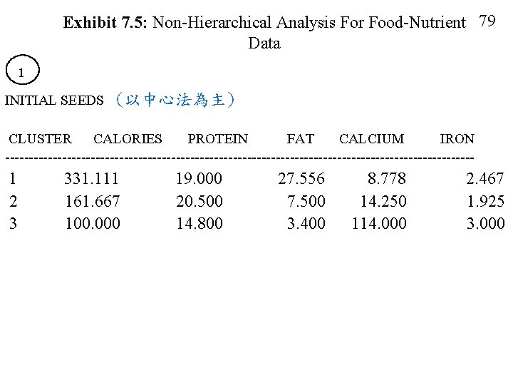
Exhibit 7. 5: Non-Hierarchical Analysis For Food-Nutrient 79 Data 1 INITIAL SEEDS (以中心法為主) CLUSTER CALORIES PROTEIN FAT CALCIUM IRON -------------------------------------------------- 1 2 3 331. 111 161. 667 100. 000 19. 000 20. 500 14. 800 27. 556 7. 500 3. 400 8. 778 14. 250 114. 000 2. 467 1. 925 3. 000

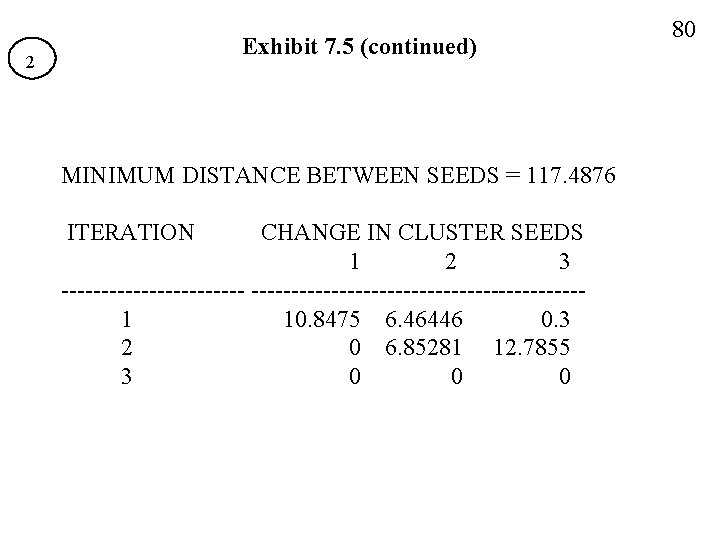
Exhibit 7. 5 (continued) 2 MINIMUM DISTANCE BETWEEN SEEDS = 117. 4876 ITERATION CHANGE IN CLUSTER SEEDS 1 2 3 --------------------------------1 10. 8475 6. 46446 0. 3 2 0 6. 85281 12. 7855 3 0 0 0 80

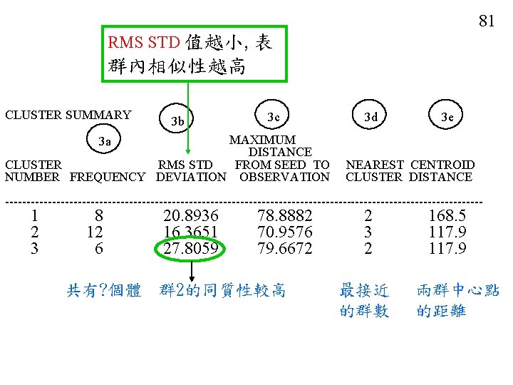
81 RMS STD 值越小, 表 群內相似性越高 CLUSTER SUMMARY 3 b 3 c MAXIMUM DISTANCE CLUSTER RMS STD FROM SEED TO NUMBER FREQUENCY DEVIATION OBSERVATION 3 d 3 e 3 a NEAREST CENTROID CLUSTER DISTANCE -------------------------------------------------------- 1 2 3 8 12 6 共有? 個體 20. 8936 16. 3651 27. 8059 78. 8882 70. 9576 79. 6672 群 2的同質性較高 2 3 2 最接近 的群數 168. 5 117. 9 兩群中心點 的距離

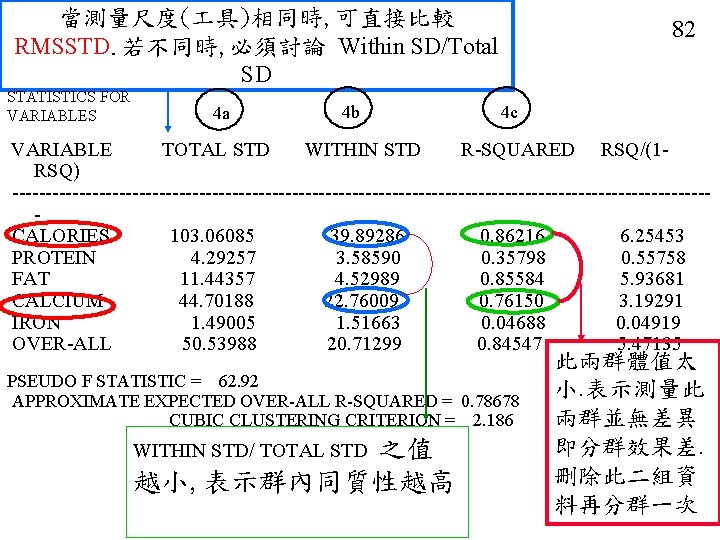
當測量尺度( 具)相同時, 可直接比較 RMSSTD. 若不同時, 必須討論 Within SD/Total SD STATISTICS FOR VARIABLES 4 a 4 b 82 4 c VARIABLE TOTAL STD WITHIN STD R-SQUARED RSQ/(1 RSQ) ----------------------------------------------------CALORIES 103. 06085 39. 89286 0. 86216 6. 25453 PROTEIN 4. 29257 3. 58590 0. 35798 0. 55758 FAT 11. 44357 4. 52989 0. 85584 5. 93681 CALCIUM 44. 70188 22. 76009 0. 76150 3. 19291 IRON 1. 49005 1. 51663 0. 04688 0. 04919 OVER-ALL 50. 53988 20. 71299 0. 84547 5. 47135 PSEUDO F STATISTIC = 62. 92 APPROXIMATE EXPECTED OVER-ALL R-SQUARED = 0. 78678 CUBIC CLUSTERING CRITERION = 2. 186 之值 越小, 表示群內同質性越高 WITHIN STD/ TOTAL STD 此兩群體值太 小. 表示測量此 兩群並無差異 即分群效果差. 刪除此二組資 料再分群一次

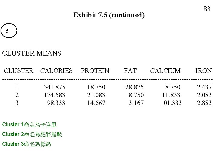
Exhibit 7. 5 (continued) 83 5 CLUSTER MEANS CLUSTER CALORIES PROTEIN FAT CALCIUM IRON -----------------------------------------------1 341. 875 18. 750 28. 875 8. 750 2. 437 2 174. 583 21. 083 8. 750 11. 833 2. 083 3 98. 333 14. 667 3. 167 101. 333 2. 883 Cluster 1命名為卡洛里 Cluster 2命名為肥胖指數 Cluster 3命名為低鈣

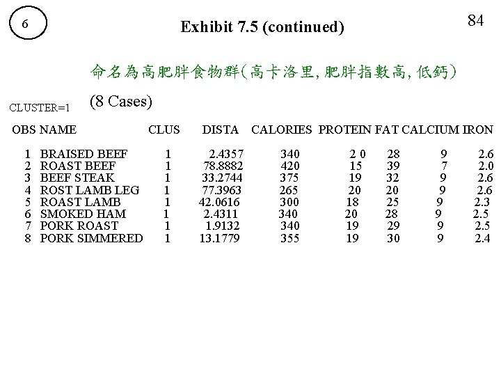
6 84 Exhibit 7. 5 (continued) 命名為高肥胖食物群(高卡洛里, 肥胖指數高, 低鈣) CLUSTER=1 (8 Cases) OBS NAME 1 2 3 4 5 6 7 8 BRAISED BEEF ROAST BEEF STEAK ROST LAMB LEG ROAST LAMB SMOKED HAM PORK ROAST PORK SIMMERED CLUS DISTA 1 1 1 1 2. 4357 78. 8882 33. 2744 77. 3963 42. 0616 2. 4311 1. 9132 13. 1779 CALORIES PROTEIN FAT CALCIUM IRON 340 420 375 265 300 340 355 20 15 19 20 18 20 19 19 28 39 32 20 25 28 29 30 9 7 9 9 9 2. 6 2. 0 2. 6 2. 3 2. 5 2. 4

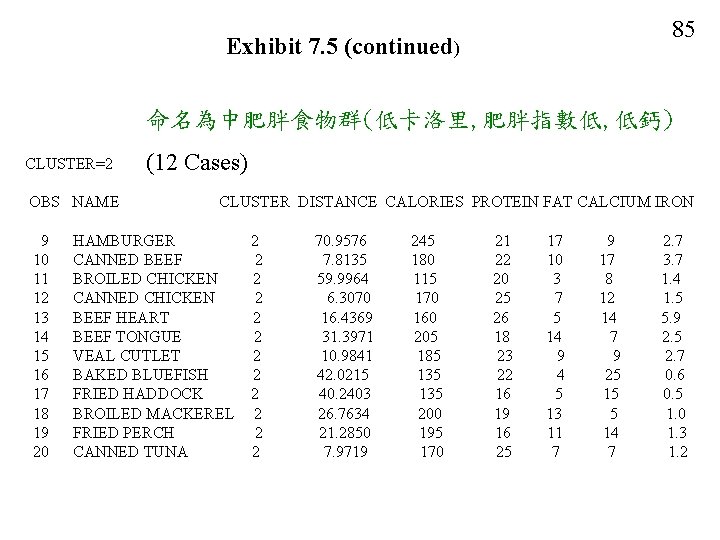
85 Exhibit 7. 5 (continued) 命名為中肥胖食物群(低卡洛里, 肥胖指數低, 低鈣) CLUSTER=2 OBS NAME 9 10 11 12 13 14 15 16 17 18 19 20 (12 Cases) CLUSTER DISTANCE CALORIES PROTEIN FAT CALCIUM IRON HAMBURGER CANNED BEEF BROILED CHICKEN CANNED CHICKEN BEEF HEART BEEF TONGUE VEAL CUTLET BAKED BLUEFISH FRIED HADDOCK BROILED MACKEREL FRIED PERCH CANNED TUNA 2 2 2 70. 9576 7. 8135 59. 9964 6. 3070 16. 4369 31. 3971 10. 9841 42. 0215 40. 2403 26. 7634 21. 2850 7. 9719 245 180 115 170 160 205 185 135 200 195 170 21 22 20 25 26 18 23 22 16 19 16 25 17 10 3 7 5 14 9 4 5 13 11 7 9 17 8 12 14 7 9 25 15 5 14 7 2. 7 3. 7 1. 4 1. 5 5. 9 2. 5 2. 7 0. 6 0. 5 1. 0 1. 3 1. 2

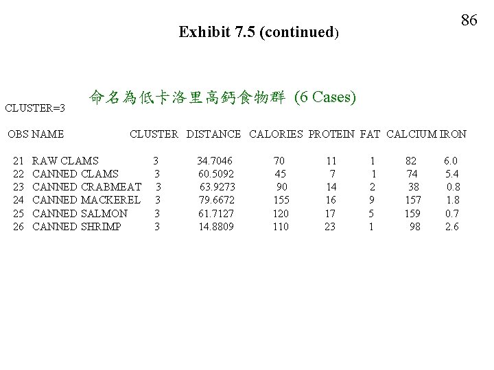
86 Exhibit 7. 5 (continued) CLUSTER=3 OBS NAME 21 22 23 24 25 26 命名為低卡洛里高鈣食物群 (6 Cases) CLUSTER DISTANCE CALORIES PROTEIN FAT CALCIUM IRON RAW CLAMS CANNED CRABMEAT CANNED MACKEREL CANNED SALMON CANNED SHRIMP 3 3 3 34. 7046 60. 5092 63. 9273 79. 6672 61. 7127 14. 8809 70 45 90 155 120 11 7 14 16 17 23 1 1 2 9 5 1 82 74 38 157 159 98 6. 0 5. 4 0. 8 1. 8 0. 7 2. 6