Principal Component Analysis CSE 4309 Machine Learning Vassilis

Principal Component Analysis CSE 4309 – Machine Learning Vassilis Athitsos Computer Science and Engineering Department University of Texas at Arlington 1

The Curse of Dimensionality • We have seen a few aspects of this curse. • As the dimensions increase, learning probability distributions becomes more difficult. – More parameters must be estimated. – More training data is needed to reliably estimate those parameters. • For example: – To learn multidimensional histograms, the number of required training data is exponential to the number of dimensions. – To learn multidimensional Gaussians, the number of required training data is quadratic to the number of dimensions. 2

The Curse of Dimensionality • There are several other aspects of the curse. • Running time can also be an issue. • Running backpropagation or decision tree learning on thousands or millions of dimensions requires more time. – For backpropagation, running time is at least linear to the number of dimensions. • It can be quadratic, if the first hidden layer has as many units as the input layer, and each hidden unit is connected to each input unit. – For decision trees, running time is linear to the number of dimensions. • Storage space is also linear to the number of dimensions. 3

Do We Need That Many Dimensions? • Consider these five images. – Each of them is a 100 x 100 grayscale image. – What is the dimensionality of each image? 4

Do We Need That Many Dimensions? • 5

Dimensionality Reduction • 6

Dimensionality Reduction • 7

Linear Dimensionality Reduction • 8

Intrinsic Dimensionality • Sometimes, high dimensional data is generated using some process that uses only a few parameters. – The translated and rotated images of the digit 3 are such an example. • In that case, the number of those few parameters is called the intrinsic dimensionality of the data. • It is desirable (but oftentimes hard) to discover the intrinsic dimensionality of the data. 9

Lossy Dimensionality Reduction • Suppose we want to project all points to a single line. • This will be lossy. • What would be the best line? 10

Lossy Dimensionality Reduction • Suppose we want to project all points to a single line. • This will be lossy. • What would be the best line? • Optimization problem. – The number of choices is infinite. – We must define an optimization criterion. 11

Optimization Criterion • 12

Optimization Criterion • 13

Optimization Criterion 14

Optimization Criterion 15

Optimization Criterion 16

Optimization Criterion: Preserving Distances 17

Optimization Criterion: Preserving Distances 18

Optimization Criterion: Preserving Distances 19

Optimization Criterion: Preserving Distances 20

Optimization Criterion: Maximizing Distances 21

Optimization Criterion: Maximizing Distances 22

Optimization Criterion: Maximizing Distances 23

Optimization Criterion: Maximizing Distances 24

Optimization Criterion: Maximizing Distances 25

Optimization Criterion: Maximizing Distances 26

Optimization Criterion: Maximizing Distances 27

Optimization Criterion: Maximizing Distances 28

Optimization Criterion: Maximizing Distances 29

Optimization Criterion: Maximizing Variance 30

Optimization Criterion: Maximizing Variance 31

Maximizing the Variance Line projection minimizing variance. Line projection maximizing variance. 32

Maximizing the Variance Line projection minimizing variance. Line projection maximizing variance. 33

Maximizing the Variance Line projection maximizing variance. 34

Maximizing the Variance Line projection maximizing variance. 35

Maximizing the Variance 36

Maximizing the Variance 37

Maximizing the Variance 38

Maximizing the Variance 39

Maximizing the Variance 40

Eigenvectors and Eigenvalues 41

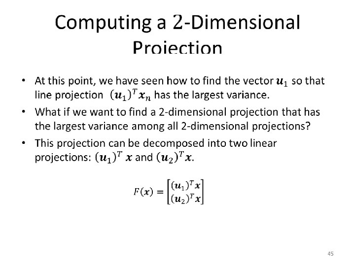
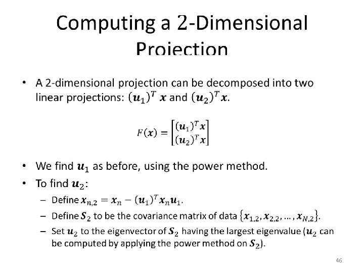
Maximizing the Variance 42

Maximizing the Variance 43

Finding the Eigenvector with the Largest Eigenvalue • 44

Projection to Orthogonal Subspace • 47

Projection to Orthogonal Subspace • 48

Projection to Orthogonal Subspace • 49

Projection to Orthogonal Subspace • 50

Projection to Orthogonal Subspace • 51

Projection to Orthogonal Subspace • 52

Projection to Orthogonal Subspace • 53

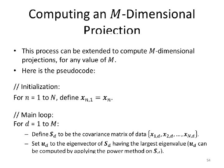
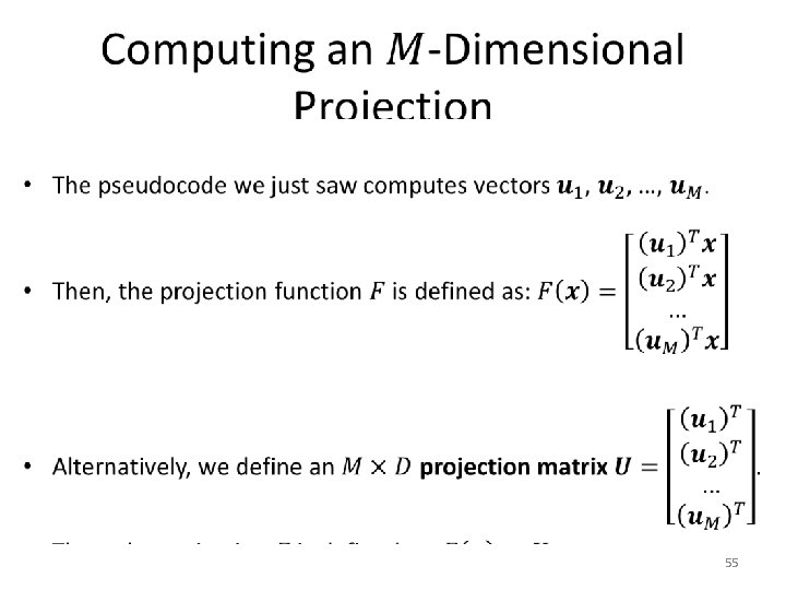
Eigenvectors • 56

Principal Component Analysis • 57

Backprojection? • 58

Backprojection? • 59

Backprojection? • We will now see a third formulation for PCA, that uses a different optimization criterion. – It ends up defining the same projection as our previous formulation. – However, this new formulation gives us an easy way to define the backprojection function. 60

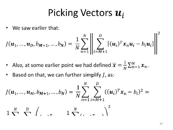
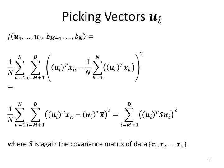
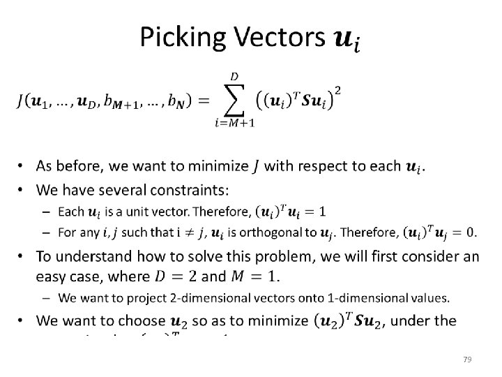
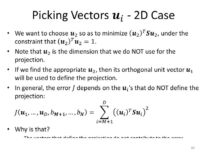
Minimum-Error Formulation • 61

Minimum-Error Formulation • 62

Minimum-Error Formulation • 63

Minimum-Error Formulation • 64

Minimum-Error Formulation • 65

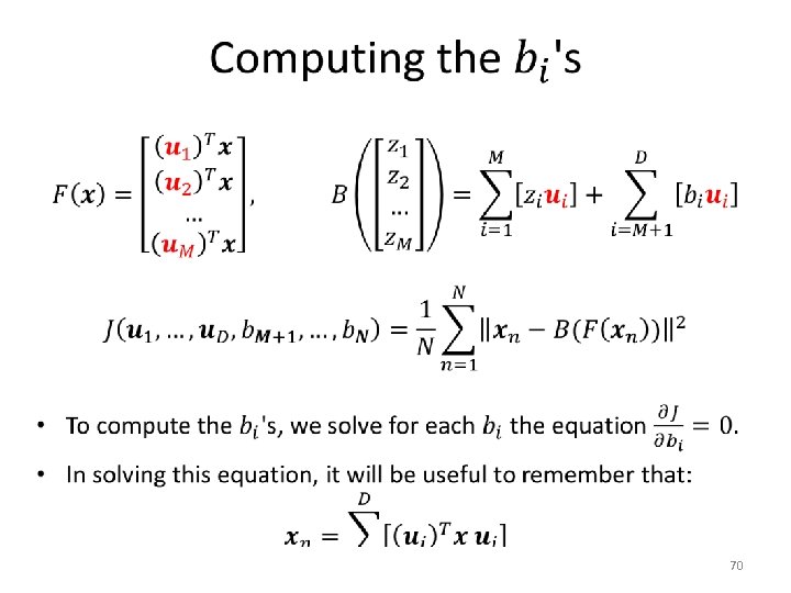
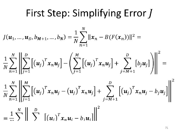
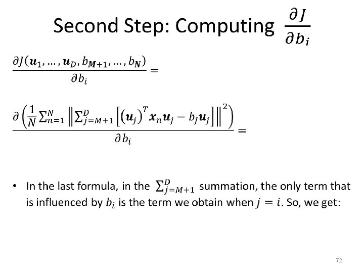
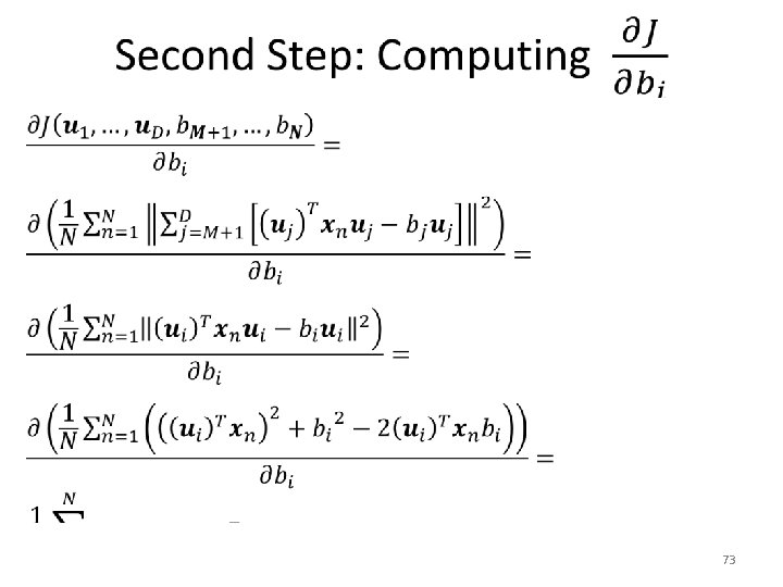
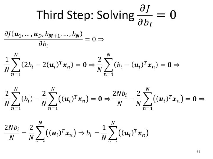
Minimum-Error Formulation • 67

Minimum-Error Formulation • 68

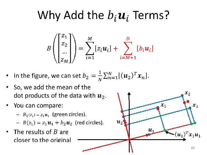
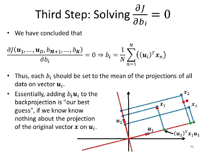
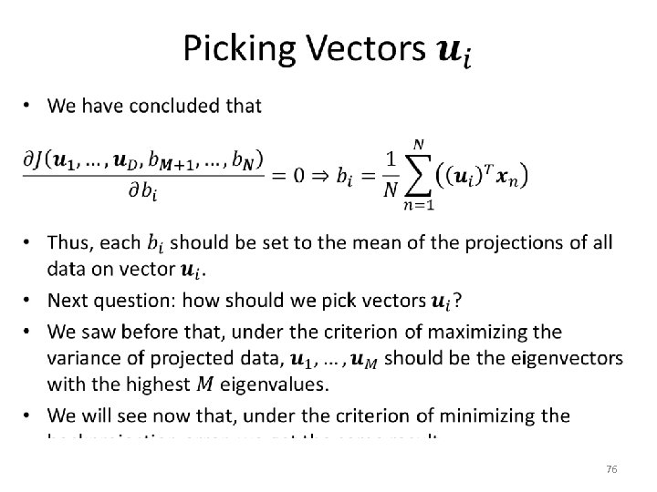
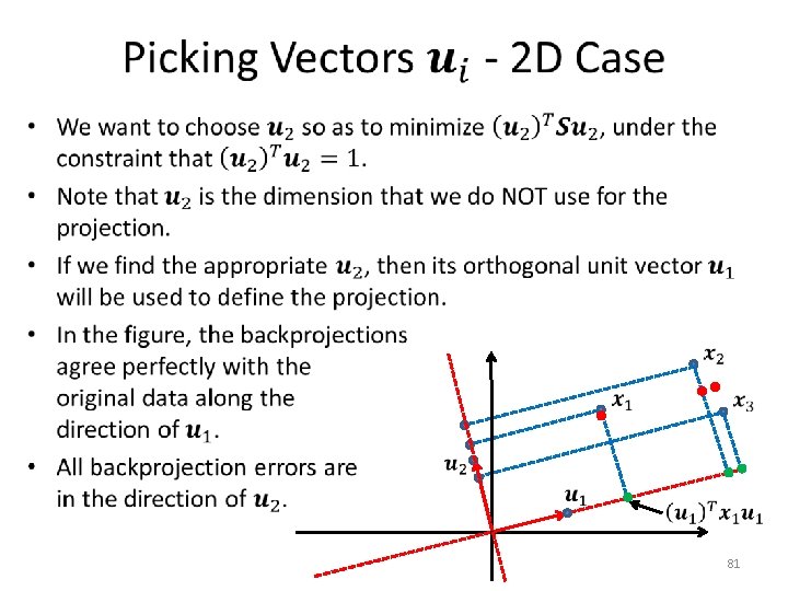
Backprojection Error • 69

PCA Recap • 86

PCA Recap • 87

Time Complexity of PCA • 88

Example Application: PCA on Faces •

Example Application: PCA on Faces •

Visualizing Eigenfaces • Eigenfaces is a computer vision term, referring to the top eigenvectors of a face dataset. • Here are the top 4 eigenfaces. • A face can be mapped to only 4 dimensions, by taking its dot product with these 4 eigenfaces. • We will see in a bit how well that works.

Visualizing Eigenfaces • Eigenfaces is a computer vision term, referring to the top eigenvectors of a face dataset. • Here are the eigenfaces ranked 5 to 8.

Approximating a Face With 0 Numbers • What is the best approximation we can get for a face image, if we know nothing about the face image (except that it is a face)?

Equivalent Question in 2 D • What is our best guess for a 2 D point from this point cloud, if we know nothing about that 2 D point (except that it belongs to the cloud)? Answer: the average of all points in the cloud.

Approximating a Face With 0 Numbers • What is the best approximation we can get for a face image, if we know nothing about the face image (except that it is a face)?

Approximating a Face With 0 Numbers • What is the best approximation we can get for a face image, if we know nothing about the face image (except that it is a face)? – The average face.

Guessing a 2 D Point Given 1 Number • What is our best guess for a 2 D point from this point cloud, if we know nothing about that 2 D point, except a single number? – What should that number be?

Guessing a 2 D Point Given 1 Number • What is our best guess for a 2 D point from this point cloud, if we know nothing about that 2 D point, except a single number? – What should that number be? – Answer: the projection on the first eigenvector.

Approximating a Face With 1 Number • What is the best approximation we can get for a face image, if we can represent the face with a single number? Average face

Approximating a Face With 1 Number • With 0 numbers, we get the average face. • With 1 number: – We map each face to its dot product with the top eigenface. – Here is the backprojection of that 1 D projection:

Approximating a Face With 2 Numbers • We map each face to a 2 D vector, using its dot products with the top 2 eigenfaces. • Here is the backprojection of that projection:

Approximating a Face With 3 Numbers • We map each face to a 3 D vector, using its dot products with the top 3 eigenfaces. • Here is the backprojection of that projection:

Approximating a Face With 4 Numbers • We map each face to a 4 D vector, using its dot products with the top 4 eigenfaces. • Here is the backprojection of that projection:

Approximating a Face With 5 Numbers • We map each face to a 5 D vector, using its dot products with the top 5 eigenfaces. • Here is the backprojection of that projection:

Approximating a Face With 6 Numbers • We map each face to a 6 D vector, using its dot products with the top 6 eigenfaces. • Here is the backprojection of that projection:

Approximating a Face With 7 Numbers • We map each face to a 7 D vector, using its dot products with the top 7 eigenfaces. • Here is the backprojection of that projection:

Approximating a Face With 10 Numbers • We map each face to a 10 D vector, using its dot products with the top 10 eigenfaces. • Here is the backprojection of that projection:

Backprojection Results original 10 eigenfaces 40 eigenfaces 100 eigenfaces

Backprojection Results original 10 eigenfaces 40 eigenfaces 100 eigenfaces

Backprojection Results original 10 eigenfaces 40 eigenfaces Note: teeth not visible using 10 eigenfaces 100 eigenfaces

Backprojection Results original 10 eigenfaces 40 eigenfaces 100 eigenfaces Note: using 10 eigenfaces, gaze direction is towards camera

Backprojection Results original 10 eigenfaces 40 eigenfaces Note: using 10 eigenfaces, glasses are removed 100 eigenfaces

Projecting a Non-Face original 10 eigenfaces 40 eigenfaces 100 eigenfaces The backprojection looks much more like a face than the original image.

Projecting a Half Face face with no occlusion occluded bottom half (input to PCA) With 10 eigenfaces, the reconstruction looks quite a bit like a regular face. reconstruction of picture with occluded bottom half, using 10 eigenfaces

Projecting a Half Face face with no occlusion occluded bottom half (input to PCA projection) With 100 eigenfaces, the reconstruction starts resembling the original input to the PCA projection. The more eigenfaces we use, the more the reconstruction resembles the original input. reconstruction of picture with occluded bottom half, using 100 eigenfaces

How Much Can 10 Numbers Tell? original Which image on the right shows the same person as the original image? Backprojections of 10 -dimensional PCA projections.

How Much Can 10 Numbers Tell? original Which image on the right shows the same person as the original image? Backprojections of 10 -dimensional PCA projections.

Uses of PCA • PCA can be a part of many different pattern recognition pipelines. • It can be used to preprocess the data before learning probability distributions, using for example histograms, Gaussians, or mixtures of Gaussians. • It can be used as a basis function, preprocessing input before applying one of the methods we have studied, like linear regression/classification, neural networks, decision trees, … 118

PCA Applications: Face Detection • A common approach for detecting faces is to: – Build a classifier that decides, given an image window, if it is a face or not. – Apply this classifier on (nearly) every possible window in the image, of every possible center and scale. – Return as detected faces the windows where the classifier output is above a certain threshold (or below a certain threshold, depending on how the classifier is defined). 119

PCA Applications: Face Detection • A common approach for detecting faces is to: – Build a classifier that decides, given an image window, if it is a face or not. – Apply this classifier on (nearly) every possible window in the image, of every possible center and scale. – Return as detected faces the windows where the classifier output is above a certain threshold (or below a certain threshold, depending on how the classifier is defined). For example: • Set scale to 20 x 20 • Apply the classifier on every image window of that scale. 120

PCA Applications: Face Detection • A common approach for detecting faces is to: – Build a classifier that decides, given an image window, if it is a face or not. – Apply this classifier on (nearly) every possible window in the image, of every possible center and scale. – Return as detected faces the windows where the classifier output is above a certain threshold (or below a certain threshold, depending on how the classifier is defined). • Set scale to 25 x 25 • Apply the classifier on every image window of that scale. 121

PCA Applications: Face Detection • A common approach for detecting faces is to: – Build a classifier that decides, given an image window, if it is a face or not. – Apply this classifier on (nearly) every possible window in the image, of every possible center and scale. – Return as detected faces the windows where the classifier output is above a certain threshold (or below a certain threshold, depending on how the classifier is defined). • Set scale to 30 x 30 • Apply the classifier on every image window of that scale. 122

PCA Applications: Face Detection • A common approach for detecting faces is to: – Build a classifier that decides, given an image window, if it is a face or not. – Apply this classifier on (nearly) every possible window in the image, of every possible center and scale. – Return as detected faces the windows where the classifier output is above a certain threshold (or below a certain threshold, depending on how the classifier is defined). • And so on, up to scales that are as large as the original image. 123

PCA Applications: Face Detection • A common approach for detecting faces is to: – Build a classifier that decides, given an image window, if it is a face or not. – Apply this classifier on (nearly) every possible window in the image, of every possible center and scale. – Return as detected faces the windows where the classifier output is above a certain threshold (or below a certain threshold, depending on how the classifier is defined). • Finally, output the windows for which the classifier output was above a threshold. – Some may be right, some may be wrong. 124

PCA Applications: Face Detection • 125

PCA Applications: Pattern Classification • Consider the satellite dataset. – Each vector in that dataset has 36 dimensions. • A PCA projection on 2 dimensions keeps 86% of the variance of the training data. • A PCA projection on 5 dimensions keeps 94% of the variance of the training data. • A PCA projection on 7 dimensions keeps 97% of the variance of the training data. 126

PCA Applications: Pattern Classification • Consider the satellite dataset. • What would work better, from the following options? – Bayes classifier using 36 -dimensional Gaussians. – Bayes classifier using 7 -dimensional Gaussians computed from PCA output. – Bayes classifier using 5 -dimensional Gaussians computed from PCA output. – Bayes classifier using 2 -dimensional histogram computed from PCA output. 127

PCA Applications: Pattern Classification • We cannot really predict which one would work better, without doing experiments. • PCA loses some information. – That may lead to higher classification error compared to using the original data as input to the classifier. • Defining Gaussians and histograms on lowerdimensional spaces requires fewer parameters. – Those parameters can be estimated more reliably from limited training data. – That may lead to lower classification error, compared to using the original data as input to the classifier. 128

Variations and Alternatives to PCA • There exist several alternatives for dimensionality reduction. • We will mention a few, but in very little detail. • Variations of PCA: – Probabilistic PCA. – Kernel PCA. • Alternatives to PCA: – – Autoencoders. Multidimensional scaling (we will not discuss). Isomap (we will not discuss). Locally linear embedding (we will not discuss). 129

Probabilistic PCA • 130

Kernel PCA • 131

Autoencoders 0 or more hidden layers • 0 or more hidden layers 132

Autoencoders 0 or more hidden layers • 0 or more hidden layers 133

Autoencoders 0 or more hidden layers • 0 or more hidden layers 134

Autoencoders 0 or more hidden layers • 0 or more hidden layers 135