KMeans Segmentation Segmentation Pictures from Mean Shift A

K-Means Segmentation

Segmentation

* * Pictures from Mean Shift: A Robust Approach toward Feature Space Analysis, by D. Comaniciu and P. Meer http: //www. caip. rutgers. edu/~comanici/MSPAMI/ms. Pami. Results. html

Segmentation and Grouping • Motivation: not information is evidence • Obtain a compact representation from an image/motion sequence/set of tokens • Should support application • Broad theory is absent at present • Grouping (or clustering) – collect together tokens that “belong together” • Fitting – associate a model with tokens – issues • which model? • which token goes to which element? • how many elements in the model?

General ideas • tokens – whatever we need to group (pixels, points, surface elements, etc. ) • top down segmentation – tokens belong together because they lie on the same object • bottom up segmentation – tokens belong together because they are locally coherent • These two are not mutually exclusive

Why do these tokens belong together?

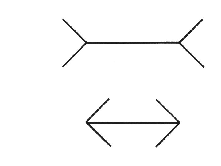
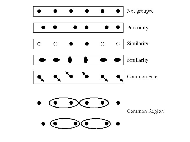
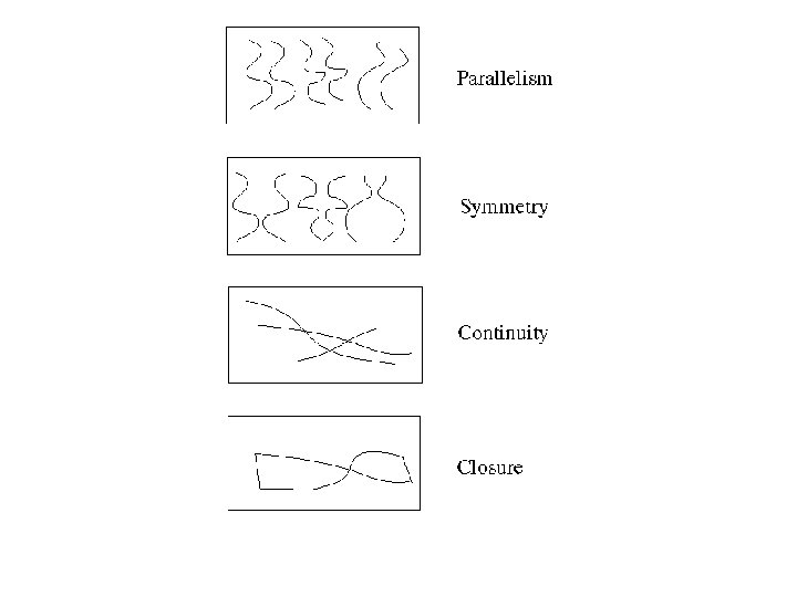
Basic ideas of grouping in humans • Figure-ground discrimination – grouping can be seen in terms of allocating some elements to a figure, some to ground – impoverished theory • Gestalt properties – elements in a collection of elements can have properties that result from relationships (Muller -Lyer effect) • gestaltqualitat – A series of factors affect whether elements should be grouped together • Gestalt factors

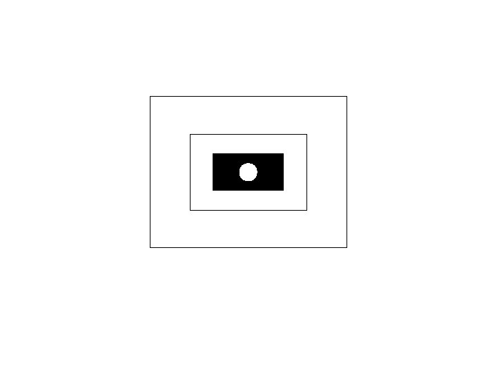
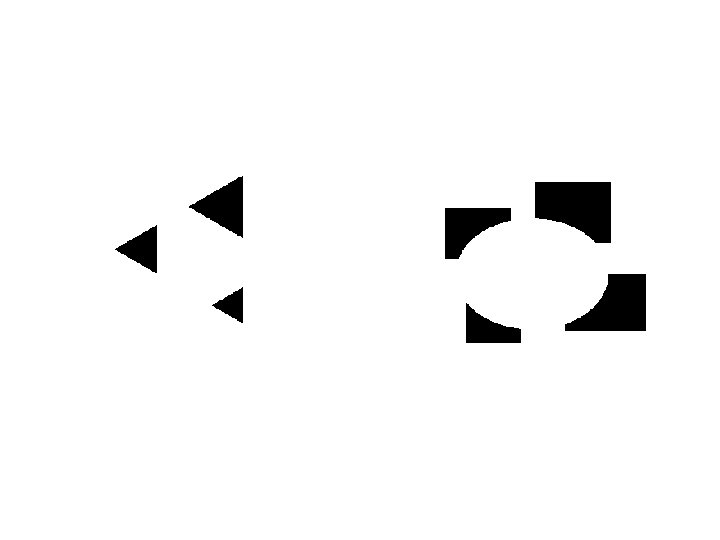
Groupings by Invisible Completions

Here, the 3 D nature of grouping is apparent: Why do these tokens belong together? Corners and creases in 3 D, length is interpreted differently: In Out University of Missouri at Columbia The (in) line at the far end of corridor must be longer than the (out) near line if they measure to be the same size

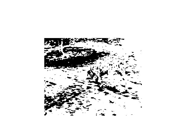
And the famous invisible dog eating under a tree:

A Final Example

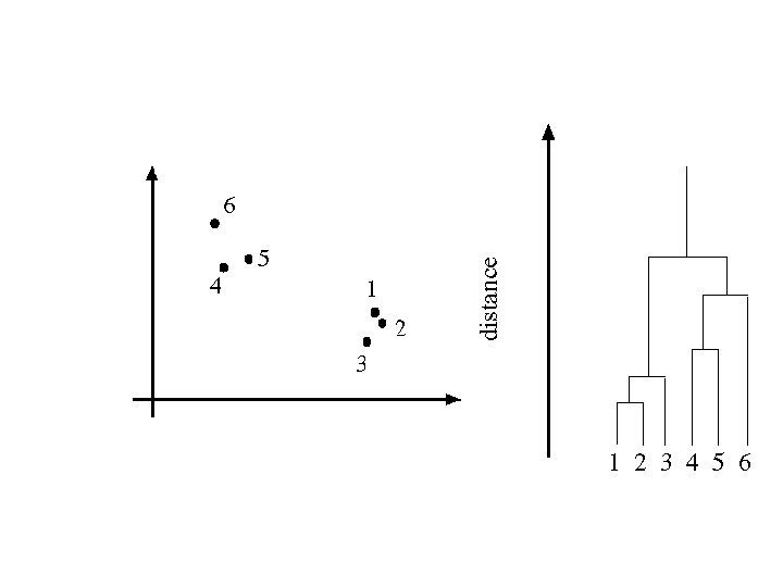
Segmentation as clustering • Cluster together (pixels, tokens, etc. ) that belong together • Agglomerative clustering – attach closest to cluster it is closest to – repeat • Divisive clustering – split cluster along best boundary – repeat • Point-Cluster distance – single-link clustering – complete-link clustering – group-average clustering • Dendrograms – yield a picture of output as clustering process continues

Simple clustering algorithms

K-Means • Choose a fixed number of • clusters Algorithm – • • Choose cluster centers and point-cluster allocations to minimize error can’t do this by search, • because there are too many possible allocations. – fix cluster centers; allocate points to closest cluster fix allocation; compute best cluster centers x could be any set of features for which we can compute a distance (careful about scaling) * From Marc Pollefeys COMP 256 2003

K-Means

K-Means * From Marc Pollefeys COMP 256 2003

Image Segmentation by K-Means • • • Select a value of K Select a feature vector for every pixel (color, texture, position, or combination of these etc. ) Define a similarity measure between feature vectors (Usually Euclidean Distance). Apply K-Means Algorithm. Apply Connected Components Algorithm. Merge any components of size less than some threshold to an adjacent component that is most similar to it. * From Marc Pollefeys COMP 256 2003

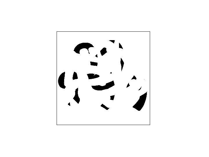
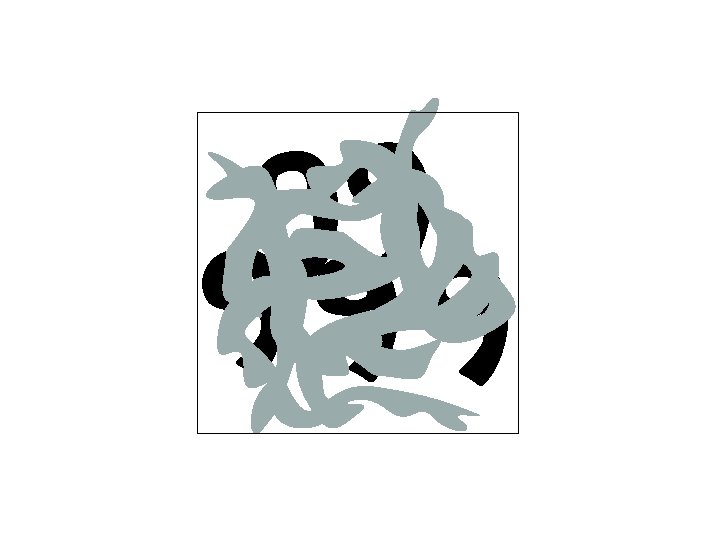
Results of K-Means Clustering: Image Clusters on intensity Clusters on color K-means clustering using intensity alone and color alone

K-Means • Is an approximation to EM – Model (hypothesis space): Mixture of N Gaussians – Latent variables: Correspondence of data and Gaussians • We notice: – Given the mixture model, it’s easy to calculate the correspondence – Given the correspondence it’s easy to estimate the mixture models

Generalized K-Means (EM)

K-Means • Choose a fixed number of clusters • Choose cluster centers and point-cluster allocations to minimize error • can’t do this by search, because there are too many possible allocations. University of Missouri at Columbia

Image Clusters on color K-means using color alone, 11 segments

K-means using color alone, 11 segments.

K-means using colour and position, 20 segments

Graph theoretic clustering • Represent tokens (which are associated with each pixel) using a weighted graph. – affinity matrix (pij has affinity of 0) • Cut up this graph to get subgraphs with strong interior links and weaker exterior links

Graphs Representations a c b e d Adjacency Matrix: W

Weighted Graphs a b c e 6 d Weight Matrix: W

Minimum Cut A cut of a graph G is the set of edges S such that removal of S from G disconnects G. Minimum cut is the cut of minimum weight, where weight of cut <A, B> is given as

Minimum Cut and Clustering

Image Segmentation & Minimum Cut Pixel Neighborhood Image Pixels w Similarity Measure Minimum Cut

Minimum Cut • There can be more than one minimum cut in a given graph • All minimum cuts of a graph can be found in polynomial time 1.

Finding the Minimal Cuts: Spectral Clustering Overview Data Similarities Block. Detection

Eigenvectors and Blocks • Block matrices have block eigenvectors: 1 1 0 0 0 0 1 1 eigensolver • Near-block matrices have nearblock eigenvectors: [Ng et al. , NIPS 02] 1 1 . 2 0 1 1 0 -. 2 1 1 eigensolver 1= 2 2= 2 . 71 0 0 . 71 1= 2. 02 2= 2. 02 . 71 0 . 69 -. 14 . 69 0 . 71 3= 0 3= -0. 02 4= 0 4= -0. 02

Spectral Space • Can put items into blocks by eigenvectors: 1 1 . 2 0 . 71 0 1 1 0 -. 2 . 69 -. 14 . 2 0 1 1 . 14 . 69 0 -. 2 1 1 0 . 71 e 2 e 1 e 2 • Resulting clusters independent of row ordering: e 1 1 . 2 1 0 . 71 0 . 2 1 0 1 . 14 . 69 1 0 1 -. 2 . 69 -. 14 0 1 -. 2 1 0 . 71 e 2 e 2

The Spectral Advantage • The key advantage of spectral clustering is the spectral space representation:

Clustering and Classification • Once our data is in spectral space: – Clustering – Classification

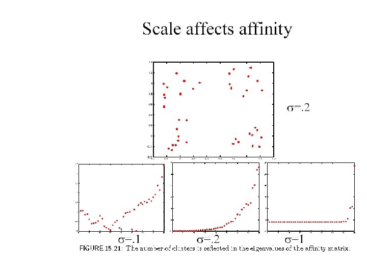
Measuring Affinity Intensity Distance Texture

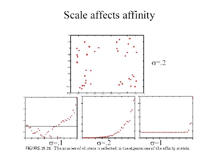
Scale affects affinity

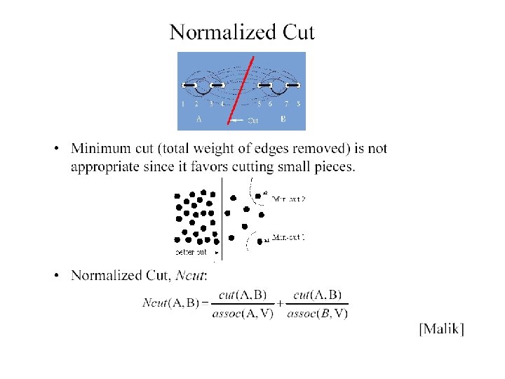
Drawbacks of Minimum Cut • Weight of cut is directly proportional to the number of edges in the cut. Cuts with lesser weight than the ideal cut Ideal Cut

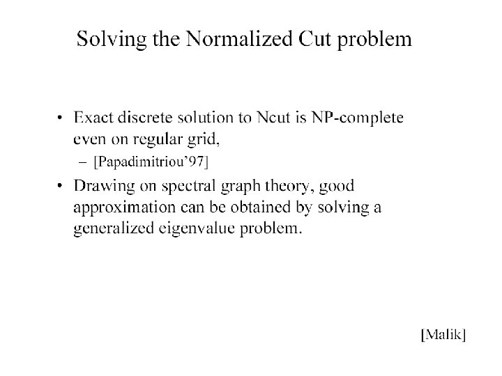
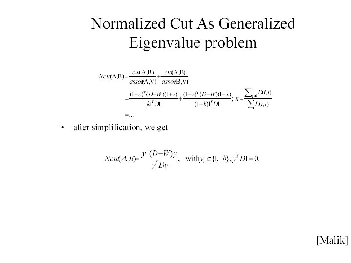
Normalized Cuts 1 • Normalized cut is defined as • Ncut(A, B) is the measure of dissimilarity of sets A and B. • Small if – Weights between clusters small – Weights within a cluster large • Minimizing Ncut(A, B) maximizes a measure of similarity within the sets A and B

Finding Minimum Normalized-Cut • Finding the Minimum Normalized-Cut is NPHard. • Polynomial Approximations are generally used for segmentation

Finding Minimum Normalized-Cut

Finding Minimum Normalized-Cut • It can be shown that such that • If y is allowed to take real values then the minimization can be done by solving the generalized eigenvalue system

Algorithm • • Compute matrices W & D Solve for eigen vectors with the smallest eigen values Use the eigen vector with second smallest eigen value to bipartition the graph Recursively partition the segmented parts if necessary.

Example eigenvector points matrix eigenvector

More than two segments • Two options – Recursively split each side to get a tree, continuing till the eigenvalues are too small – Use the other eigenvectors

More than two segments

Normalized cuts • Current criterion evaluates within cluster similarity, but not across cluster difference • Instead, we’d like to maximize the within cluster similarity compared to the across cluster difference • Write graph as V, one cluster as A and the other as B • Maximize • i. e. construct A, B such that their within cluster similarity is high compared to their association with the rest of the graph

Figure from “Image and video segmentation: the normalised cut framework”, by Shi and Malik, copyright IEEE, 1998

Figure from “Normalized cuts and image segmentation, ” Shi and Malik, copyright IEEE, 2000

Drawbacks of Minimum Normalized Cut • Huge Storage Requirement and time complexity • Bias towards partitioning into equal segments • Have problems with textured backgrounds