Stat Quest http www statquest com Stat Quest

Stat. Quest! http: //www. statquest. com

Stat. Quest! http: //www. statquest. com

Stat. Quest! http: //www. statquest. com

Heatmaps… • You’ve seen them before…. http: //www. statquest. com

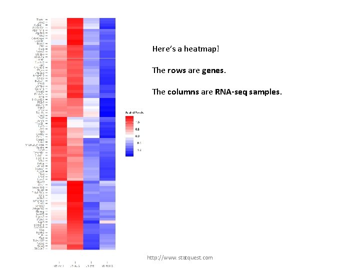
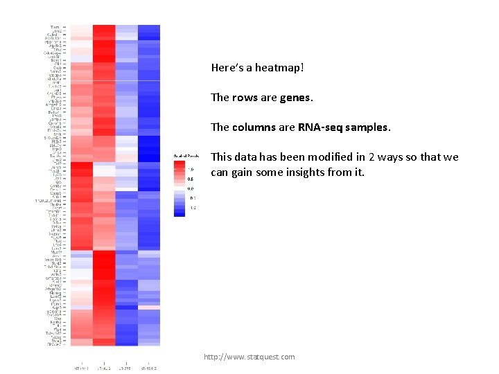
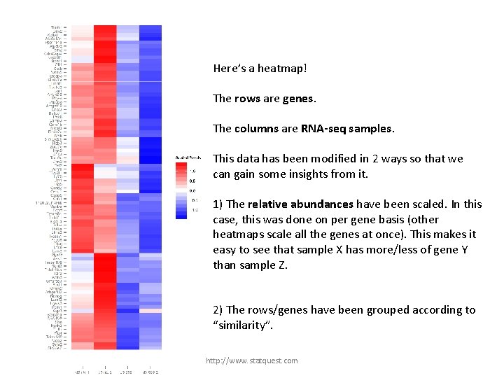
Here’s a heatmap! The rows are genes. The columns are RNA-seq samples. http: //www. statquest. com

Here’s a heatmap! The rows are genes. The columns are RNA-seq samples. This data has been modified in 2 ways so that we can gain some insights from it. http: //www. statquest. com

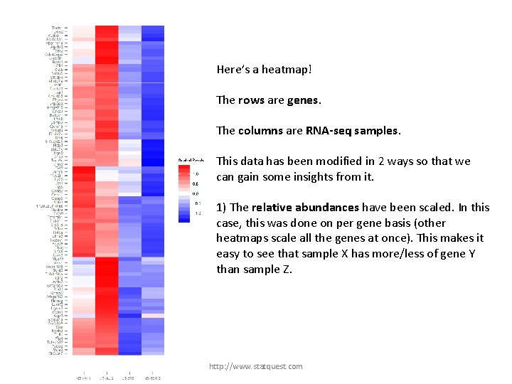
Here’s a heatmap! The rows are genes. The columns are RNA-seq samples. This data has been modified in 2 ways so that we can gain some insights from it. 1) The relative abundances have been scaled. In this case, this was done on per gene basis (other heatmaps scale all the genes at once). This makes it easy to see that sample X has more/less of gene Y than sample Z. http: //www. statquest. com

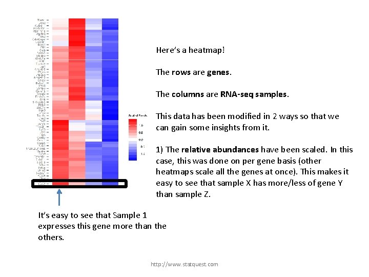
Here’s a heatmap! The rows are genes. The columns are RNA-seq samples. This data has been modified in 2 ways so that we can gain some insights from it. 1) The relative abundances have been scaled. In this case, this was done on per gene basis (other heatmaps scale all the genes at once). This makes it easy to see that sample X has more/less of gene Y than sample Z. It’s easy to see that Sample 1 expresses this gene more than the others. http: //www. statquest. com

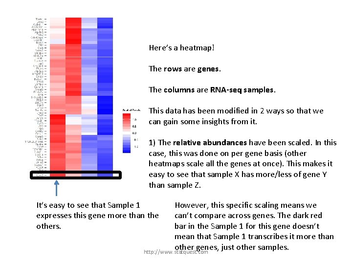
Here’s a heatmap! The rows are genes. The columns are RNA-seq samples. This data has been modified in 2 ways so that we can gain some insights from it. 1) The relative abundances have been scaled. In this case, this was done on per gene basis (other heatmaps scale all the genes at once). This makes it easy to see that sample X has more/less of gene Y than sample Z. It’s easy to see that Sample 1 expresses this gene more than the others. However, this specific scaling means we can’t compare across genes. The dark red bar in the Sample 1 for this gene doesn’t mean that Sample 1 transcribes it more than other genes, just other samples. http: //www. statquest. com

Here’s a heatmap! The rows are genes. The columns are RNA-seq samples. This data has been modified in 2 ways so that we can gain some insights from it. 1) The relative abundances have been scaled. In this case, this was done on per gene basis (other heatmaps scale all the genes at once). This makes it easy to see that sample X has more/less of gene Y than sample Z. 2) The rows/genes have been grouped according to “similarity”. http: //www. statquest. com

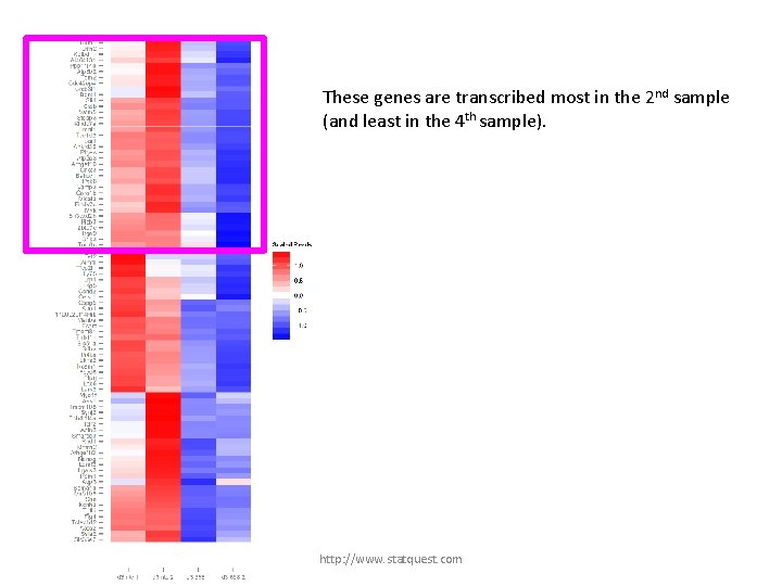
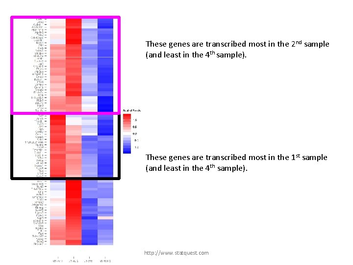
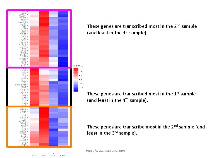
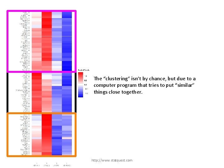
These genes are transcribed most in the 2 nd sample (and least in the 4 th sample). http: //www. statquest. com

These genes are transcribed most in the 2 nd sample (and least in the 4 th sample). These genes are transcribed most in the 1 st sample (and least in the 4 th sample). http: //www. statquest. com

These genes are transcribed most in the 2 nd sample (and least in the 4 th sample). These genes are transcribed most in the 1 st sample (and least in the 4 th sample). These genes are transcribe most in the 2 nd sample (and least in the 3 rd sample). http: //www. statquest. com

The “clustering” isn’t by chance, but due to a computer program that tries to put “similar” things close together. http: //www. statquest. com

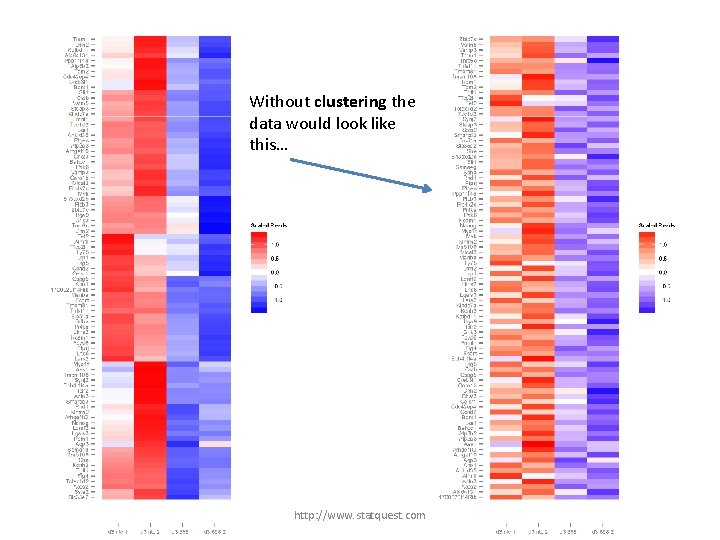
Without clustering the data would look like this… http: //www. statquest. com

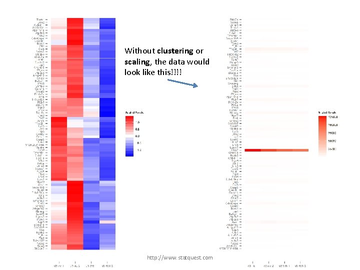
Without clustering or scaling, the data would look like this!!!! http: //www. statquest. com

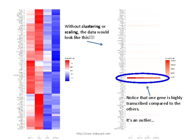
Without clustering or scaling, the data would look like this!!!! Notice that one gene is highly transcribed compared to the others. It’s an outlier… http: //www. statquest. com

Another example… http: //www. statquest. com

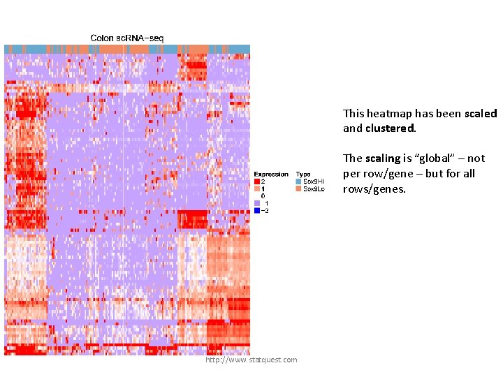
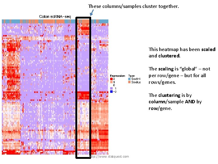
This heatmap has been scaled and clustered. The scaling is “global” – not per row/gene – but for all rows/genes. http: //www. statquest. com

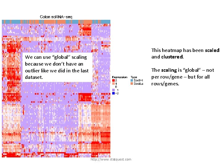
This heatmap has been scaled and clustered. We can use “global” scaling because we don’t have an outlier like we did in the last dataset. The scaling is “global” – not per row/gene – but for all rows/genes. http: //www. statquest. com

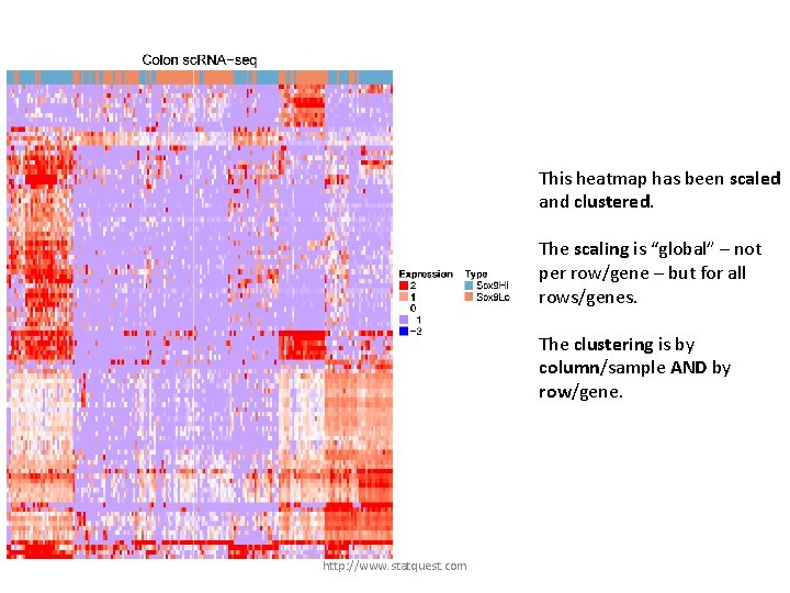
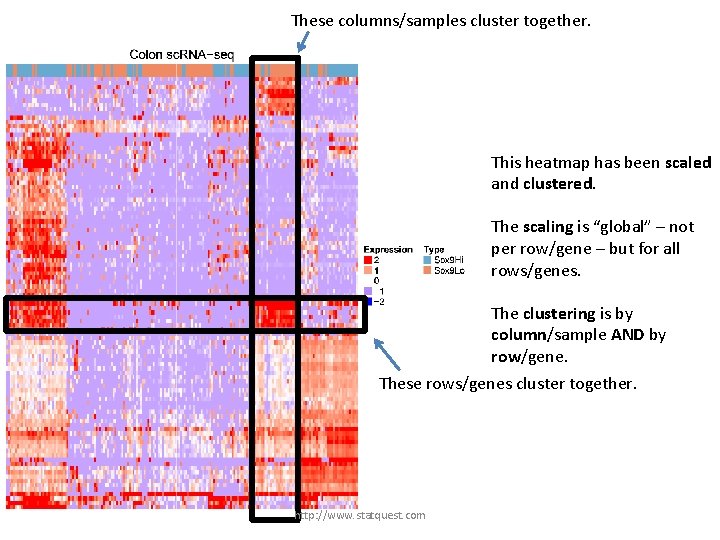
This heatmap has been scaled and clustered. The scaling is “global” – not per row/gene – but for all rows/genes. The clustering is by column/sample AND by row/gene. http: //www. statquest. com

These columns/samples cluster together. This heatmap has been scaled and clustered. The scaling is “global” – not per row/gene – but for all rows/genes. The clustering is by column/sample AND by row/gene. http: //www. statquest. com

These columns/samples cluster together. This heatmap has been scaled and clustered. The scaling is “global” – not per row/gene – but for all rows/genes. The clustering is by column/sample AND by row/gene. These rows/genes cluster together. http: //www. statquest. com

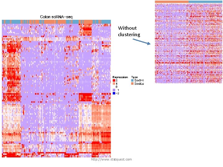
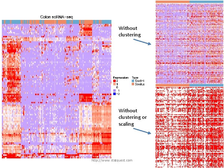
Without clustering http: //www. statquest. com

Without clustering or scaling http: //www. statquest. com

A quick aside. . http: //www. statquest. com

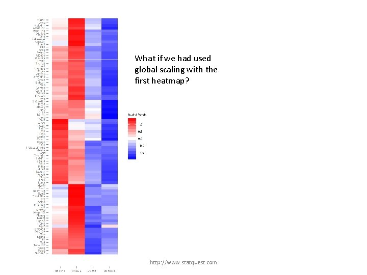
What if we had used global scaling with the first heatmap? http: //www. statquest. com

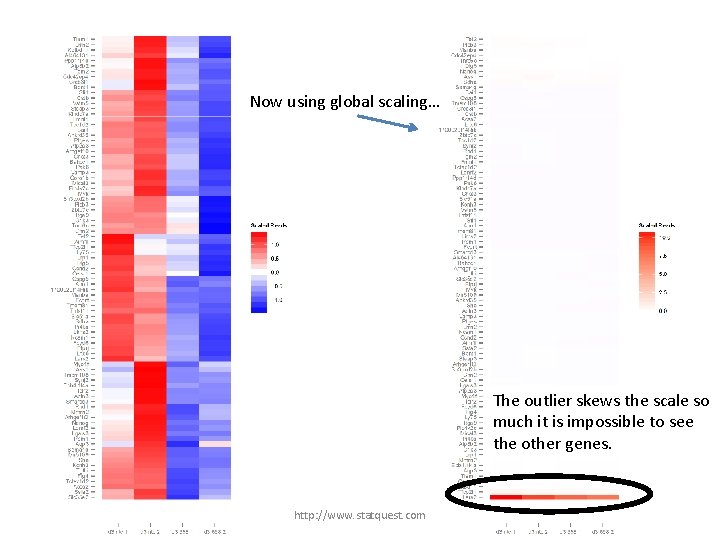
Now using global scaling… The outlier skews the scale so much it is impossible to see the other genes. http: //www. statquest. com

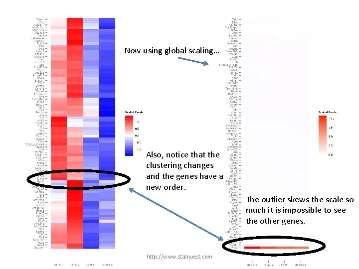
Now using global scaling… Also, notice that the clustering changes and the genes have a new order. The outlier skews the scale so much it is impossible to see the other genes. http: //www. statquest. com

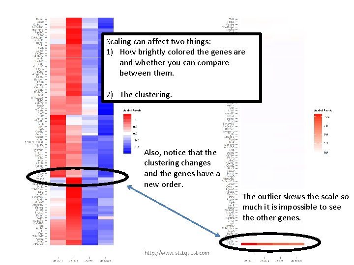
Scaling can affect two things: Nowbrightly using global scaling… 1) How colored the genes are and whether you can compare between them. 2) The clustering. Also, notice that the clustering changes and the genes have a new order. The outlier skews the scale so much it is impossible to see the other genes. http: //www. statquest. com

… now back to the action. http: //www. statquest. com

How to scale data… • Regardless of whether you do it by gene or globally, the most common method is… nameless! I hate to coin a new term, but let’s call it “Z-Score Scaling” because, technically, it converts the data to “Z-scores” http: //www. statquest. com

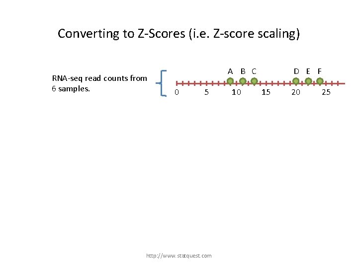
Converting to Z-Scores (i. e. Z-score scaling) RNA-seq read counts from 6 samples. A B C 0 5 http: //www. statquest. com 10 D E F 15 20 25

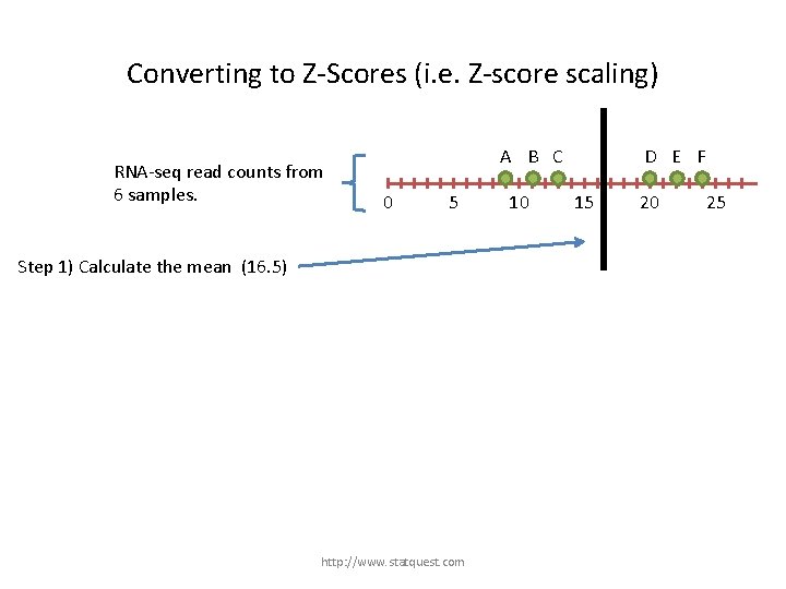
Converting to Z-Scores (i. e. Z-score scaling) RNA-seq read counts from 6 samples. A B C 0 5 Step 1) Calculate the mean (16. 5) http: //www. statquest. com 10 D E F 15 20 25

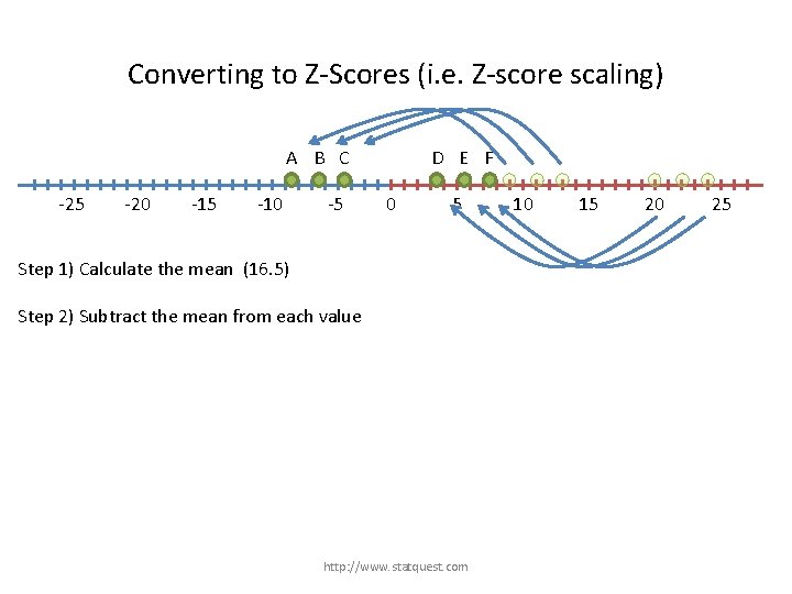
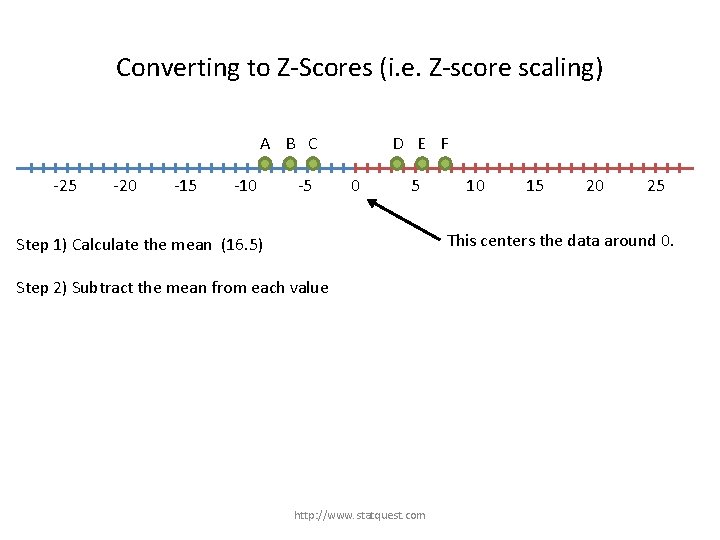
Converting to Z-Scores (i. e. Z-score scaling) A B C -25 -20 -15 -10 -5 D E F 0 5 Step 1) Calculate the mean (16. 5) Step 2) Subtract the mean from each value http: //www. statquest. com 10 15 20 25

Converting to Z-Scores (i. e. Z-score scaling) A B C -25 -20 -15 -10 -5 D E F 0 5 10 15 20 25 This centers the data around 0. Step 1) Calculate the mean (16. 5) Step 2) Subtract the mean from each value http: //www. statquest. com

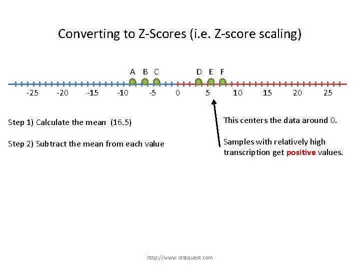
Converting to Z-Scores (i. e. Z-score scaling) A B C -25 -20 -15 -10 -5 D E F 0 5 10 15 20 25 Step 1) Calculate the mean (16. 5) This centers the data around 0. Step 2) Subtract the mean from each value Samples with relatively high transcription get positive values. http: //www. statquest. com

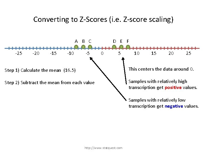
Converting to Z-Scores (i. e. Z-score scaling) A B C -25 -20 -15 -10 -5 D E F 0 5 10 15 20 25 Step 1) Calculate the mean (16. 5) This centers the data around 0. Step 2) Subtract the mean from each value Samples with relatively high transcription get positive values. Samples with relatively low transcription get negative values. http: //www. statquest. com

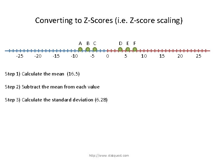
Converting to Z-Scores (i. e. Z-score scaling) A B C -25 -20 -15 -10 -5 D E F 0 5 Step 1) Calculate the mean (16. 5) Step 2) Subtract the mean from each value Step 3) Calculate the standard deviation (6. 28) http: //www. statquest. com 10 15 20 25

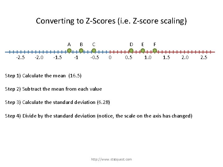
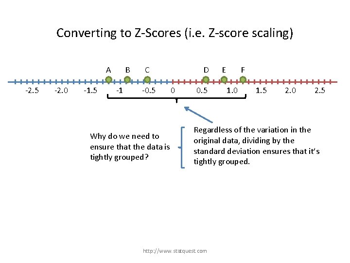
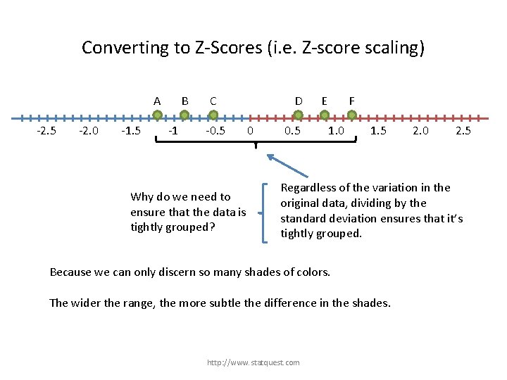
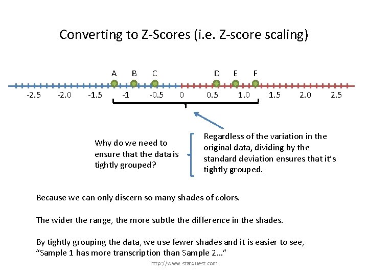
Converting to Z-Scores (i. e. Z-score scaling) A -2. 5 -2. 0 -1. 5 B -1 C -0. 5 D 0 0. 5 E F 1. 0 1. 5 2. 0 Step 1) Calculate the mean (16. 5) Step 2) Subtract the mean from each value Step 3) Calculate the standard deviation (6. 28) Step 4) Divide by the standard deviation (notice, the scale on the axis has changed) http: //www. statquest. com 2. 5

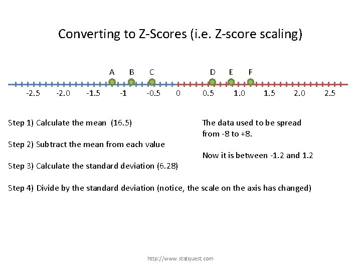
Converting to Z-Scores (i. e. Z-score scaling) A -2. 5 -2. 0 -1. 5 B -1 C -0. 5 D 0 Step 1) Calculate the mean (16. 5) Step 2) Subtract the mean from each value Step 3) Calculate the standard deviation (6. 28) 0. 5 E F 1. 0 1. 5 2. 0 The data used to be spread from -8 to +8. Now it is between -1. 2 and 1. 2 Step 4) Divide by the standard deviation (notice, the scale on the axis has changed) http: //www. statquest. com 2. 5

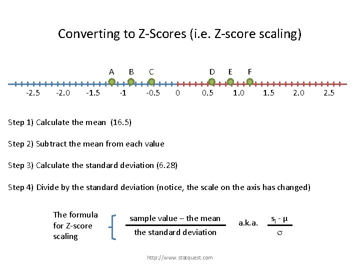
Converting to Z-Scores (i. e. Z-score scaling) A -2. 5 -2. 0 -1. 5 B -1 C -0. 5 D 0 0. 5 E F 1. 0 1. 5 2. 0 Step 1) Calculate the mean (16. 5) Step 2) Subtract the mean from each value Step 3) Calculate the standard deviation (6. 28) Step 4) Divide by the standard deviation (notice, the scale on the axis has changed) The formula for Z-score scaling sample value – the mean the standard deviation http: //www. statquest. com a. k. a. si - µ s 2. 5

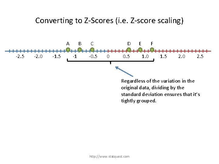
Converting to Z-Scores (i. e. Z-score scaling) A -2. 5 -2. 0 -1. 5 B -1 C -0. 5 D 0 0. 5 E F 1. 0 1. 5 2. 0 2. 5 Regardless of the variation in the original data, dividing by the standard deviation ensures that it’s tightly grouped. http: //www. statquest. com

Converting to Z-Scores (i. e. Z-score scaling) A -2. 5 -2. 0 -1. 5 B -1 C -0. 5 Why do we need to ensure that the data is tightly grouped? D 0 0. 5 E F 1. 0 1. 5 2. 0 2. 5 Regardless of the variation in the original data, dividing by the standard deviation ensures that it’s tightly grouped. http: //www. statquest. com

Converting to Z-Scores (i. e. Z-score scaling) A -2. 5 -2. 0 -1. 5 B -1 C -0. 5 Why do we need to ensure that the data is tightly grouped? D 0 0. 5 E F 1. 0 1. 5 2. 0 2. 5 Regardless of the variation in the original data, dividing by the standard deviation ensures that it’s tightly grouped. Because we can only discern so many shades of colors. The wider the range, the more subtle the difference in the shades. http: //www. statquest. com

Converting to Z-Scores (i. e. Z-score scaling) A -2. 5 -2. 0 -1. 5 B -1 C -0. 5 Why do we need to ensure that the data is tightly grouped? D 0 0. 5 E F 1. 0 1. 5 2. 0 2. 5 Regardless of the variation in the original data, dividing by the standard deviation ensures that it’s tightly grouped. Because we can only discern so many shades of colors. The wider the range, the more subtle the difference in the shades. By tightly grouping the data, we use fewer shades and it is easier to see, “Sample 1 has more transcription than Sample 2…” http: //www. statquest. com

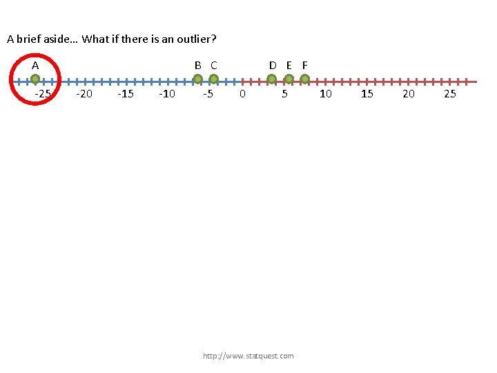
A brief aside… What if there is an outlier? http: //www. statquest. com

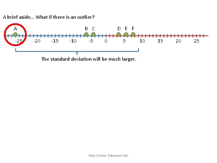
A brief aside… What if there is an outlier? A -25 B C -20 -15 -10 -5 D E F 0 5 http: //www. statquest. com 10 15 20 25

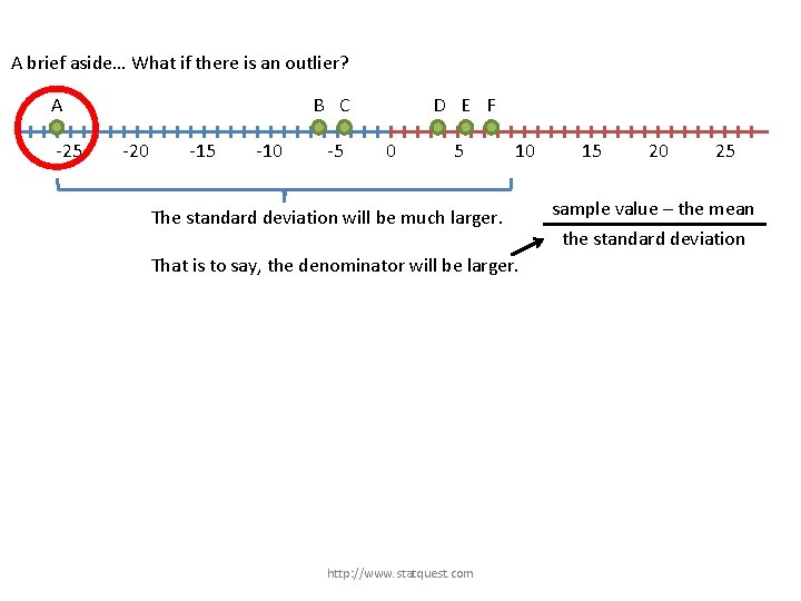
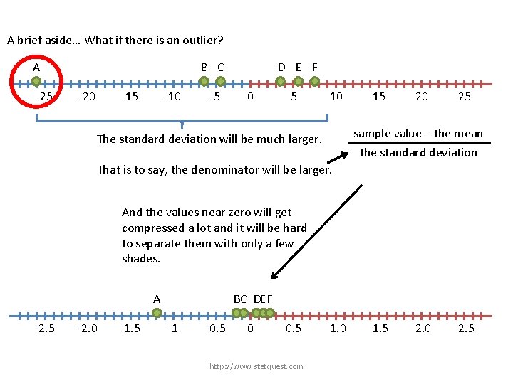
A brief aside… What if there is an outlier? A -25 B C -20 -15 -10 -5 D E F 0 5 The standard deviation will be much larger. http: //www. statquest. com 10 15 20 25

A brief aside… What if there is an outlier? A -25 B C -20 -15 -10 -5 D E F 0 5 10 The standard deviation will be much larger. That is to say, the denominator will be larger. http: //www. statquest. com 15 20 25 sample value – the mean the standard deviation

A brief aside… What if there is an outlier? A -25 B C -20 -15 -10 -5 D E F 0 5 10 15 20 25 sample value – the mean The standard deviation will be much larger. the standard deviation That is to say, the denominator will be larger. And the values near zero will get compressed a lot and it will be hard to separate them with only a few shades. A -2. 5 -2. 0 -1. 5 BC DEF -1 -0. 5 0 0. 5 http: //www. statquest. com 1. 0 1. 5 2. 0 2. 5

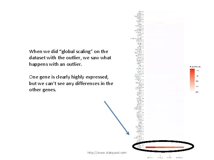
When we did “global scaling” on the dataset with the outlier, we saw what happens with an outlier. One gene is clearly highly expressed, but we can’t see any differences in the other genes. http: //www. statquest. com

Clustering – The fun part! http: //www. statquest. com

Clustering – The fun part! • There are two main types of clustering: – Hierarchical – K-means http: //www. statquest. com

Clustering – The fun part! • There are two main types of clustering: – Hierarchical – K-means • We’ll focus on hierarchical clustering for now… http: //www. statquest. com

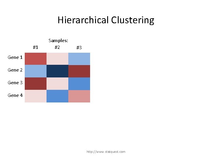
Hierarchical Clustering #1 Samples: #2 #3 Gene 1 Gene 2 Gene 3 Gene 4 http: //www. statquest. com

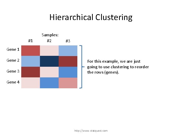
Hierarchical Clustering #1 Samples: #2 #3 Gene 1 Gene 2 Gene 3 For this example, we are just going to use clustering to reorder the rows (genes). Gene 4 http: //www. statquest. com

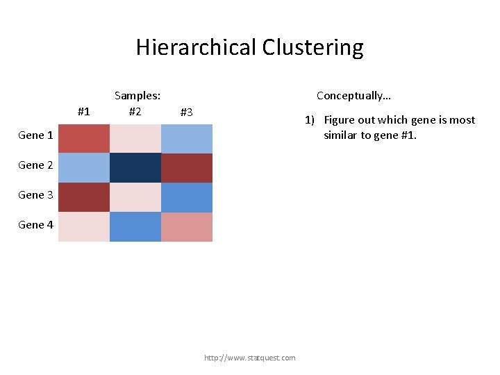
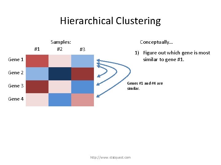
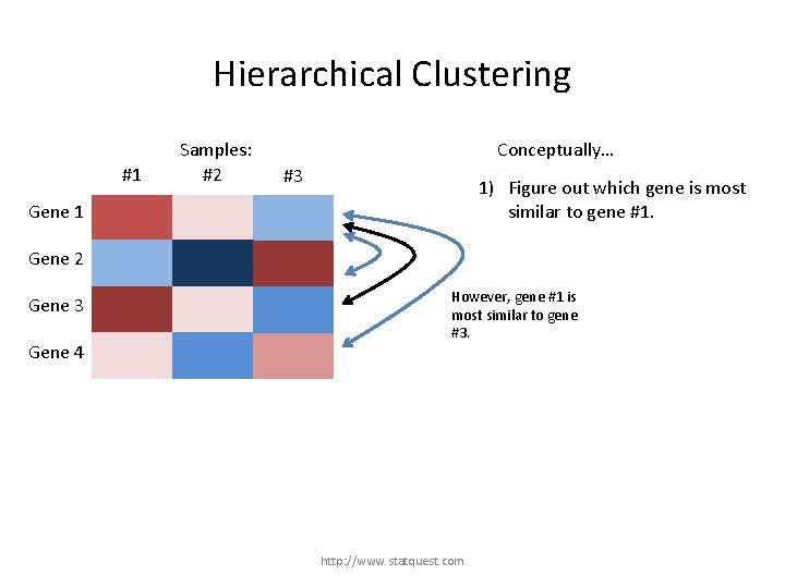
Hierarchical Clustering #1 Samples: #2 Conceptually… #3 1) Figure out which gene is most similar to gene #1. Gene 1 Gene 2 Gene 3 Gene 4 http: //www. statquest. com

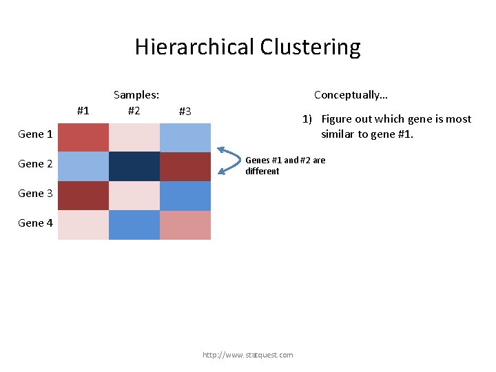
Hierarchical Clustering #1 Samples: #2 Conceptually… #3 1) Figure out which gene is most similar to gene #1. Gene 1 Gene 2 Genes #1 and #2 are different Gene 3 Gene 4 http: //www. statquest. com

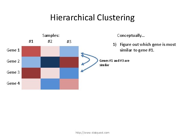
Hierarchical Clustering #1 Samples: #2 Conceptually… #3 1) Figure out which gene is most similar to gene #1. Gene 1 Gene 2 Genes #1 and #3 are similar Gene 3 Gene 4 http: //www. statquest. com

Hierarchical Clustering #1 Samples: #2 Conceptually… #3 1) Figure out which gene is most similar to gene #1. Gene 1 Gene 2 Gene 3 Genes #1 and #4 are similar. Gene 4 http: //www. statquest. com

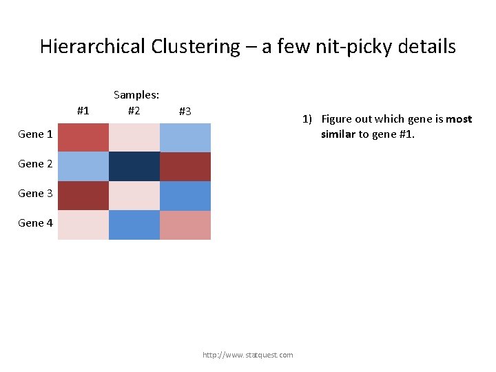
Hierarchical Clustering #1 Samples: #2 Conceptually… #3 1) Figure out which gene is most similar to gene #1. Gene 1 Gene 2 Gene 3 Gene 4 However, gene #1 is most similar to gene #3. http: //www. statquest. com

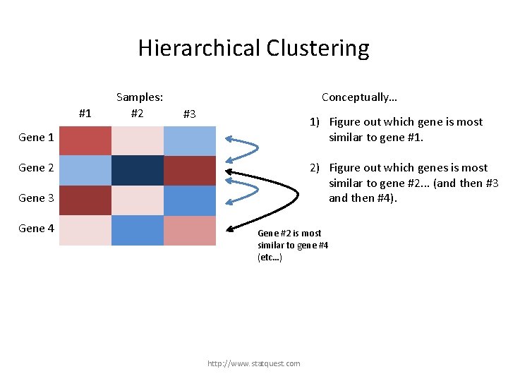
Hierarchical Clustering #1 Samples: #2 Conceptually… #3 1) Figure out which gene is most similar to gene #1. Gene 1 2) Figure out which genes is most similar to gene #2. . . (and then #3 and then #4). Gene 2 Gene 3 Gene 4 Gene #2 is most similar to gene #4 (etc…) http: //www. statquest. com

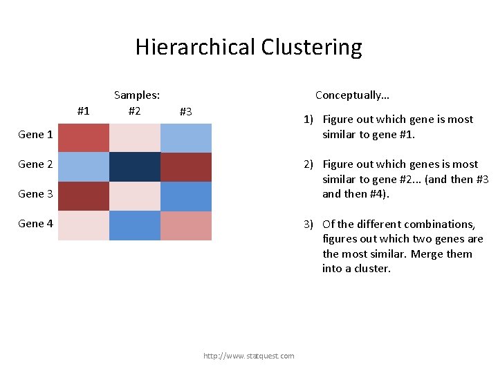
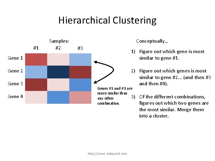
Hierarchical Clustering #1 Samples: #2 Conceptually… #3 1) Figure out which gene is most similar to gene #1. Gene 1 2) Figure out which genes is most similar to gene #2. . . (and then #3 and then #4). Gene 2 Gene 3 3) Of the different combinations, figures out which two genes are the most similar. Merge them into a cluster. Gene 4 http: //www. statquest. com

Hierarchical Clustering #1 Samples: #2 Conceptually… #3 1) Figure out which gene is most similar to gene #1. Gene 1 2) Figure out which genes is most similar to gene #2. . . (and then #3 and then #4). Gene 2 Gene 3 Gene 4 Genes #1 and #3 are more similar than 3) any other combination. http: //www. statquest. com Of the different combinations, figures out which two genes are the most similar. Merge them into a cluster.

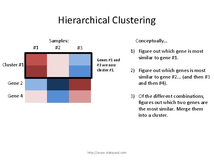
Hierarchical Clustering #1 Gene 1 Cluster #1 Gene 3 Samples: #2 Conceptually… #3 Genes #1 and #3 are now cluster #1. Gene 2 1) Figure out which gene is most similar to gene #1. 2) Figure out which genes is most similar to gene #2. . . (and then #3 and then #4). 3) Of the different combinations, figures out which two genes are the most similar. Merge them into a cluster. Gene 4 http: //www. statquest. com

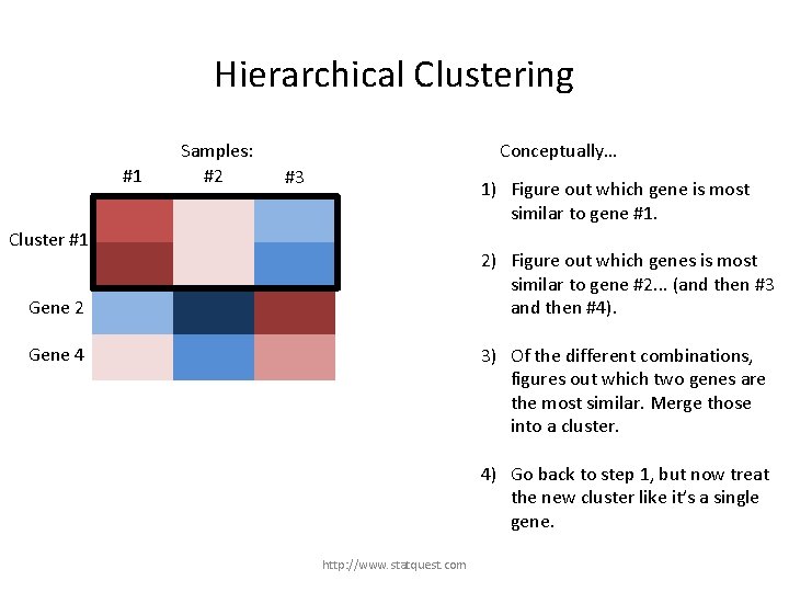
Hierarchical Clustering #1 Samples: #2 Conceptually… #3 1) Figure out which gene is most similar to gene #1. Gene 1 Cluster #1 Gene 3 2) Figure out which genes is most similar to gene #2. . . (and then #3 and then #4). Gene 2 3) Of the different combinations, figures out which two genes are the most similar. Merge those into a cluster. Gene 4 4) Go back to step 1, but now treat the new cluster like it’s a single gene. http: //www. statquest. com

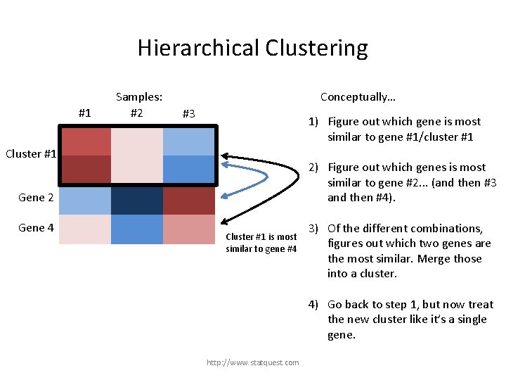
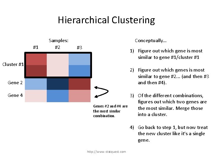
Hierarchical Clustering #1 Samples: #2 Conceptually… #3 1) Figure out which gene is most similar to gene #1/cluster #1 Gene 1 Cluster #1 Gene 3 2) Figure out which genes is most similar to gene #2. . . (and then #3 and then #4). Gene 2 Gene 4 Cluster #1 is most similar to gene #4 3) Of the different combinations, figures out which two genes are the most similar. Merge those into a cluster. 4) Go back to step 1, but now treat the new cluster like it’s a single gene. http: //www. statquest. com

Hierarchical Clustering #1 Samples: #2 Conceptually… #3 1) Figure out which gene is most similar to gene #1/cluster #1 Gene 1 Cluster #1 Gene 3 2) Figure out which genes is most similar to gene #2. . . (and then #3 and then #4). Gene 2 Gene 4 Gene #2 is most similar to gene #4 3) Of the different combinations, figures out which two genes are the most similar. Merge those into a cluster. 4) Go back to step 1, but now treat the new cluster like it’s a single gene. http: //www. statquest. com

Hierarchical Clustering #1 Samples: #2 Conceptually… #3 1) Figure out which gene is most similar to gene #1/cluster #1 Gene 1 Cluster #1 Gene 3 2) Figure out which genes is most similar to gene #2. . . (and then #3 and then #4). Gene 2 Gene 4 Genes #2 and #4 are the most similar combination. 3) Of the different combinations, figures out which two genes are the most similar. Merge those into a cluster. 4) Go back to step 1, but now treat the new cluster like it’s a single gene. http: //www. statquest. com

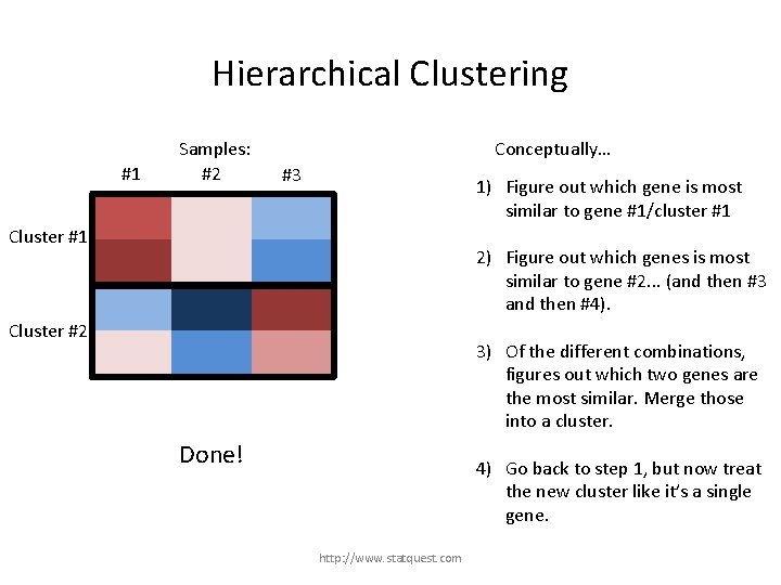
Hierarchical Clustering #1 Samples: #2 Conceptually… #3 1) Figure out which gene is most similar to gene #1/cluster #1 Cluster #1 2) Figure out which genes is most similar to gene #2. . . (and then #3 and then #4). Cluster #2 3) Of the different combinations, figures out which two genes are the most similar. Merge those into a cluster. Done! 4) Go back to step 1, but now treat the new cluster like it’s a single gene. http: //www. statquest. com

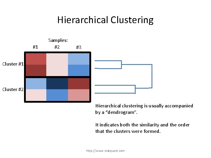
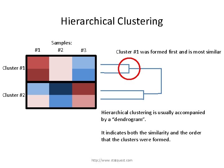
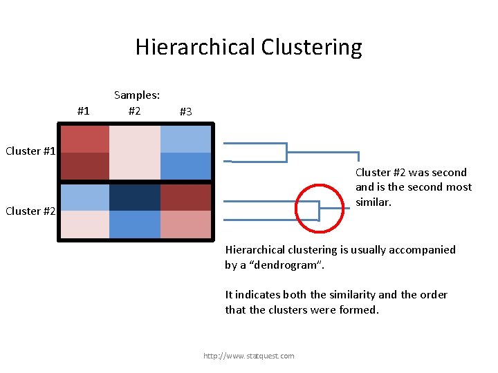
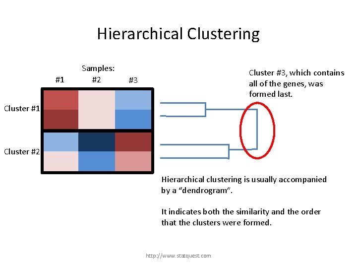
Hierarchical Clustering #1 Samples: #2 #3 Cluster #1 Cluster #2 Hierarchical clustering is usually accompanied by a “dendrogram”. It indicates both the similarity and the order that the clusters were formed. http: //www. statquest. com

Hierarchical Clustering #1 Samples: #2 #3 Cluster #1 was formed first and is most similar Cluster #1 Cluster #2 Hierarchical clustering is usually accompanied by a “dendrogram”. It indicates both the similarity and the order that the clusters were formed. http: //www. statquest. com

Hierarchical Clustering #1 Samples: #2 #3 Cluster #1 Cluster #2 was second and is the second most similar. Cluster #2 Hierarchical clustering is usually accompanied by a “dendrogram”. It indicates both the similarity and the order that the clusters were formed. http: //www. statquest. com

Hierarchical Clustering #1 Samples: #2 Cluster #3, which contains all of the genes, was formed last. #3 Cluster #1 Cluster #2 Hierarchical clustering is usually accompanied by a “dendrogram”. It indicates both the similarity and the order that the clusters were formed. http: //www. statquest. com

Hierarchical Clustering – a few nit-picky details http: //www. statquest. com

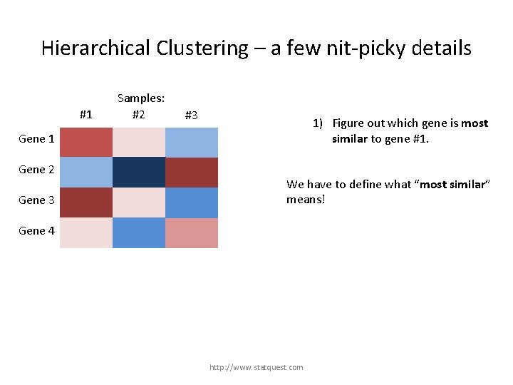
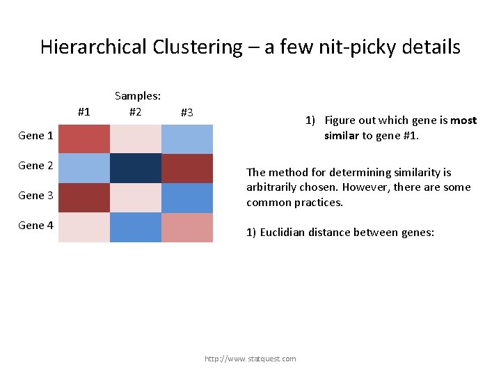
Hierarchical Clustering – a few nit-picky details #1 Samples: #2 #3 1) Figure out which gene is most similar to gene #1. Gene 1 Gene 2 Gene 3 Gene 4 http: //www. statquest. com

Hierarchical Clustering – a few nit-picky details #1 Samples: #2 #3 1) Figure out which gene is most similar to gene #1. Gene 1 Gene 2 Gene 3 We have to define what “most similar” means! Gene 4 http: //www. statquest. com

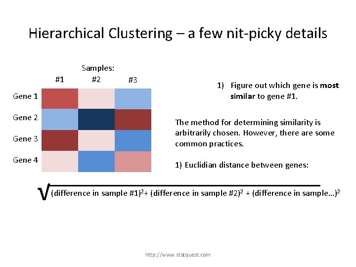
Hierarchical Clustering – a few nit-picky details #1 Samples: #2 #3 1) Figure out which gene is most similar to gene #1. Gene 1 Gene 2 Gene 3 Gene 4 The method for determining similarity is arbitrarily chosen. However, there are some common practices. 1) Euclidian distance between genes: http: //www. statquest. com

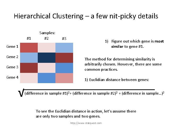
Hierarchical Clustering – a few nit-picky details #1 Samples: #2 #3 1) Figure out which gene is most similar to gene #1. Gene 1 Gene 2 The method for determining similarity is arbitrarily chosen. However, there are some common practices. Gene 3 Gene 4 1) Euclidian distance between genes: √ (difference in sample #1)2+ (difference in sample #2)2 + (difference in sample…)2 http: //www. statquest. com

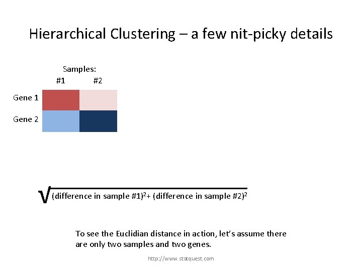
Hierarchical Clustering – a few nit-picky details #1 Samples: #2 #3 1) Figure out which gene is most similar to gene #1. Gene 1 Gene 2 The method for determining similarity is arbitrarily chosen. However, there are some common practices. Gene 3 Gene 4 1) Euclidian distance between genes: √ (difference in sample #1)2+ (difference in sample #2)2 + (difference in sample…)2 To see the Euclidian distance in action, let’s assume there are only two samples and two genes. http: //www. statquest. com

Hierarchical Clustering – a few nit-picky details Samples: #1 #2 Gene 1 Gene 2 √ (difference in sample #1)2+ (difference in sample #2)2 + (difference in sample…)2 To see the Euclidian distance in action, let’s assume there are only two samples and two genes. http: //www. statquest. com

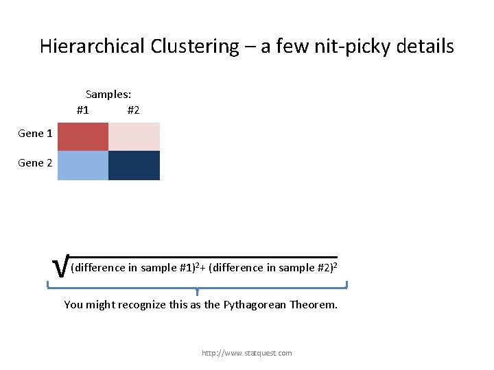
Hierarchical Clustering – a few nit-picky details Samples: #1 #2 Gene 1 Gene 2 √ (difference in sample #1)2+ (difference in sample #2)2 + (difference in gene …)2 You might recognize this as the Pythagorean Theorem. http: //www. statquest. com

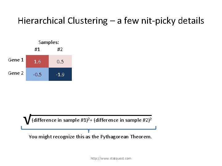
Hierarchical Clustering – a few nit-picky details Samples: #1 #2 Gene 1 1. 6 0. 5 Gene 2 -0. 5 -1. 9 √ (difference in sample #1)2+ (difference in sample #2)2 + (difference in gene …)2 You might recognize this as the Pythagorean Theorem. http: //www. statquest. com

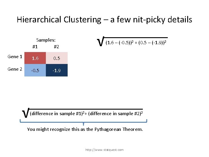
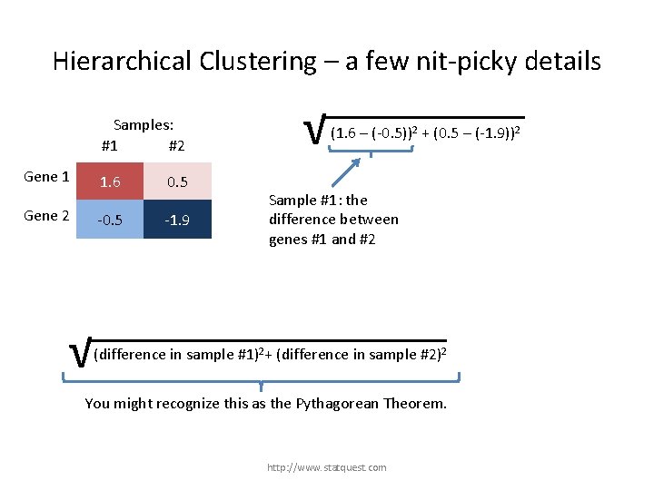
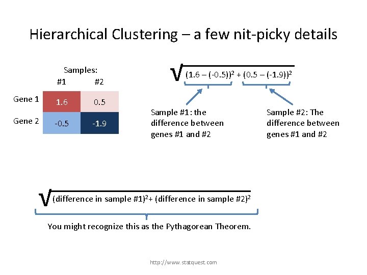
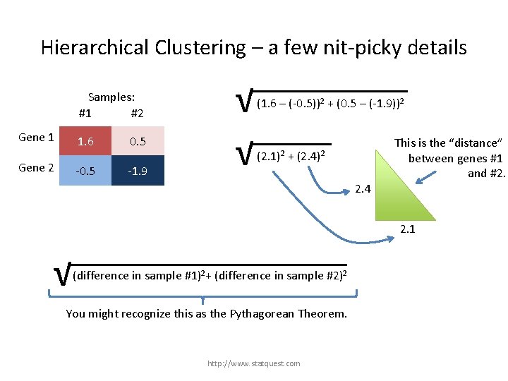
Hierarchical Clustering – a few nit-picky details Samples: #1 #2 Gene 1 1. 6 0. 5 Gene 2 -0. 5 -1. 9 √ (1. 6 – (-0. 5))2 + (0. 5 – (-1. 9))2 √ (difference in sample #1)2+ (difference in sample #2)2 + (difference in gene …)2 You might recognize this as the Pythagorean Theorem. http: //www. statquest. com

Hierarchical Clustering – a few nit-picky details Samples: #1 #2 Gene 1 Gene 2 1. 6 0. 5 -1. 9 √ (1. 6 – (-0. 5))2 + (0. 5 – (-1. 9))2 Sample #1: the difference between genes #1 and #2 √ (difference in sample #1)2+ (difference in sample #2)2 + (difference in gene …)2 You might recognize this as the Pythagorean Theorem. http: //www. statquest. com

Hierarchical Clustering – a few nit-picky details Samples: #1 #2 Gene 1 Gene 2 1. 6 0. 5 -1. 9 √ (1. 6 – (-0. 5))2 + (0. 5 – (-1. 9))2 Sample #1: the difference between genes #1 and #2 √ Sample #2: The difference between genes #1 and #2 (difference in sample #1)2+ (difference in sample #2)2 + (difference in gene …)2 You might recognize this as the Pythagorean Theorem. http: //www. statquest. com

Hierarchical Clustering – a few nit-picky details Samples: #1 #2 Gene 1 Gene 2 1. 6 0. 5 -1. 9 √ √ (1. 6 – (-0. 5))2 + (0. 5 – (-1. 9))2 (2. 1)2 + (2. 4)2 2. 4 This is the “distance” between genes #1 and #2. 2. 1 √ (difference in sample #1)2+ (difference in sample #2)2 + (difference in gene …)2 You might recognize this as the Pythagorean Theorem. http: //www. statquest. com

Hierarchical Clustering – distance metrics • Euclidian distance is just one method… there are lots more, including: – Manhattan – Canberra – etc. http: //www. statquest. com

Hierarchical Clustering – distance metrics • Euclidian distance is just one method… there are lots more, including: – Manhattan – Canberra – etc. For example, the Manhattan distance is just the absolute value of the differences…. |difference in sample #1|+ |difference in sample #2| + |difference in gene …| http: //www. statquest. com

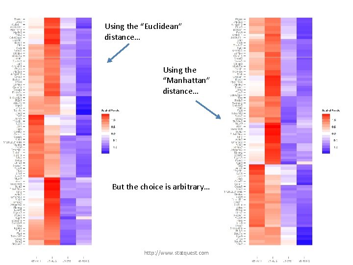
Hierarchical Clustering – distance metrics • Euclidian distance is just one method… there are lots more, including: – Manhattan – Canberra – etc. For example, the Manhattan distance is just the absolute value of the differences…. |difference in sample #1|+ |difference in sample #2| + |difference in gene …| • Yes, it makes a difference. http: //www. statquest. com

Hierarchical Clustering – distance metrics • Euclidian distance is just one method… there are lots more, including: – Manhattan – Canberra – etc. For example, the Manhattan distance is just the absolute value of the differences…. |difference in sample #1|+ |difference in sample #2| + |difference in gene …| • Yes, it makes a difference. : ( http: //www. statquest. com

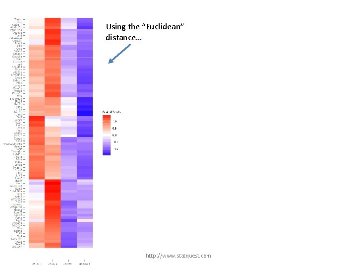
Using the “Euclidean” distance… http: //www. statquest. com

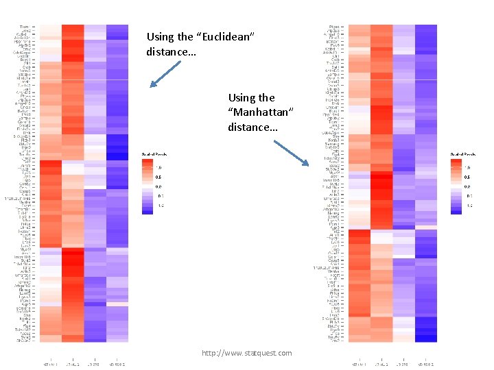
Using the “Euclidean” distance… Using the “Manhattan” distance… http: //www. statquest. com

Using the “Euclidean” distance… Using the “Manhattan” distance… But the choice is arbitrary… http: //www. statquest. com

Using the “Euclidean” distance… Using the “Manhattan” distance… But the choice is arbitrary… : ( http: //www. statquest. com

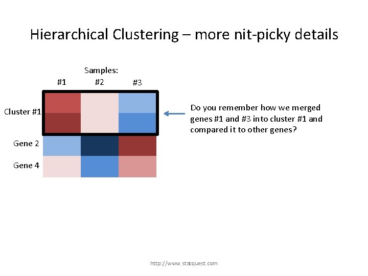
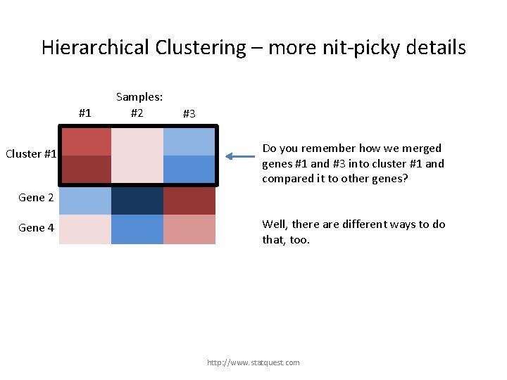
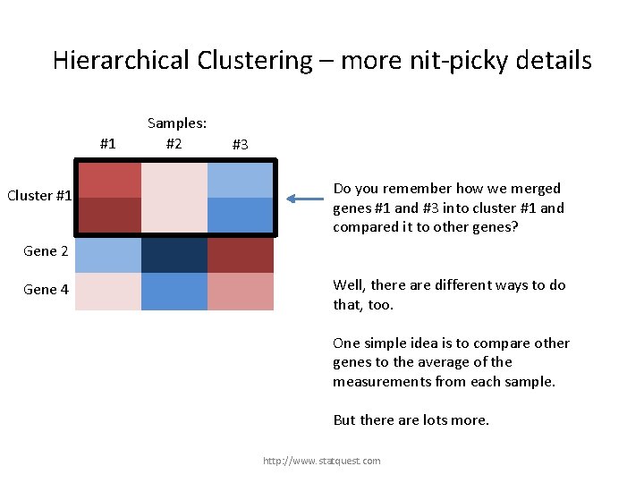
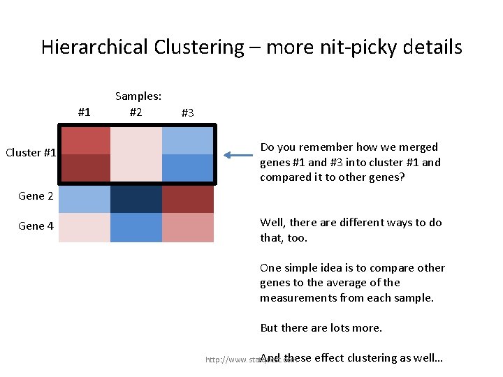
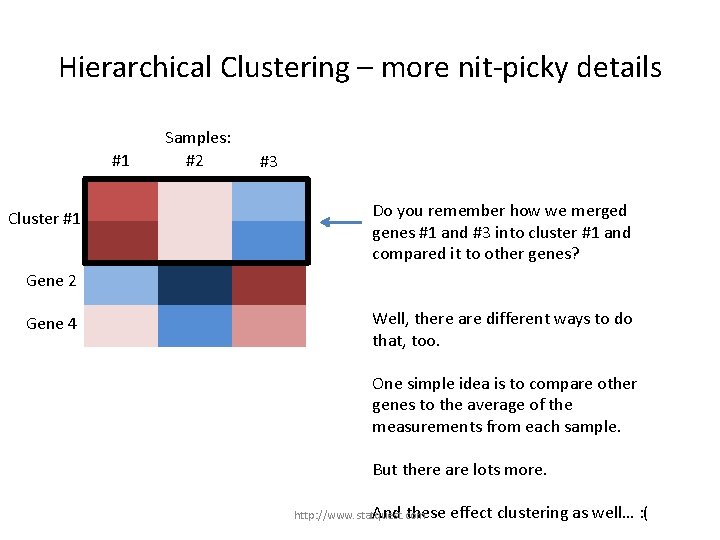
Hierarchical Clustering – more nit-picky details #1 Gene 1 Cluster #1 Gene 3 Samples: #2 #3 Do you remember how we merged genes #1 and #3 into cluster #1 and compared it to other genes? Gene 2 Gene 4 http: //www. statquest. com

Hierarchical Clustering – more nit-picky details #1 Gene 1 Cluster #1 Gene 3 Samples: #2 #3 Do you remember how we merged genes #1 and #3 into cluster #1 and compared it to other genes? Gene 2 Gene 4 Well, there are different ways to do that, too. http: //www. statquest. com

Hierarchical Clustering – more nit-picky details #1 Gene 1 Cluster #1 Gene 3 Samples: #2 #3 Do you remember how we merged genes #1 and #3 into cluster #1 and compared it to other genes? Gene 2 Gene 4 Well, there are different ways to do that, too. One simple idea is to compare other genes to the average of the measurements from each sample. But there are lots more. http: //www. statquest. com

Hierarchical Clustering – more nit-picky details #1 Gene 1 Cluster #1 Gene 3 Samples: #2 #3 Do you remember how we merged genes #1 and #3 into cluster #1 and compared it to other genes? Gene 2 Gene 4 Well, there are different ways to do that, too. One simple idea is to compare other genes to the average of the measurements from each sample. But there are lots more. And these http: //www. statquest. com effect clustering as well…

Hierarchical Clustering – more nit-picky details #1 Gene 1 Cluster #1 Gene 3 Samples: #2 #3 Do you remember how we merged genes #1 and #3 into cluster #1 and compared it to other genes? Gene 2 Gene 4 Well, there are different ways to do that, too. One simple idea is to compare other genes to the average of the measurements from each sample. But there are lots more. And these http: //www. statquest. com effect clustering as well… : (

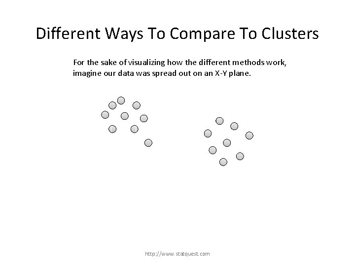
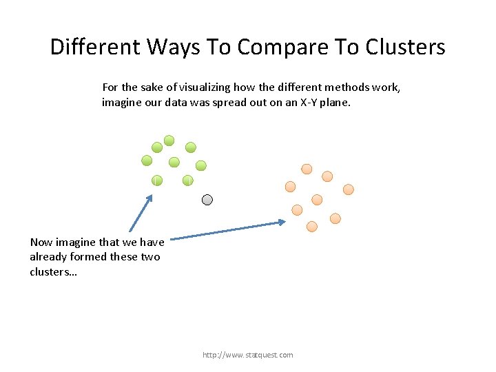
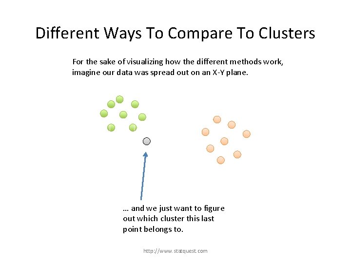
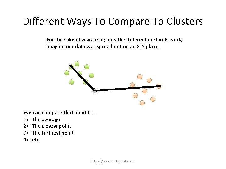
Different Ways To Compare To Clusters For the sake of visualizing how the different methods work, imagine our data was spread out on an X-Y plane. http: //www. statquest. com

Different Ways To Compare To Clusters For the sake of visualizing how the different methods work, imagine our data was spread out on an X-Y plane. Now imagine that we have already formed these two clusters… http: //www. statquest. com

Different Ways To Compare To Clusters For the sake of visualizing how the different methods work, imagine our data was spread out on an X-Y plane. … and we just want to figure out which cluster this last point belongs to. http: //www. statquest. com

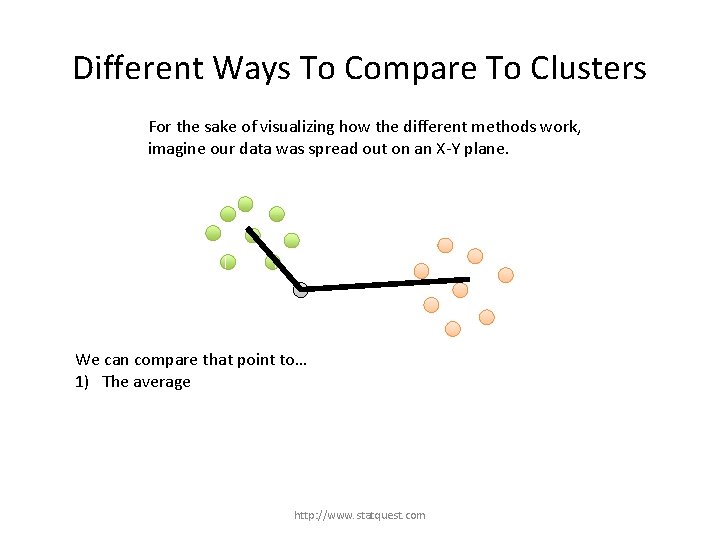
Different Ways To Compare To Clusters For the sake of visualizing how the different methods work, imagine our data was spread out on an X-Y plane. We can compare that point to… 1) The average http: //www. statquest. com

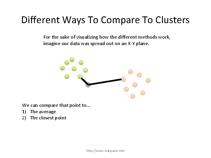
Different Ways To Compare To Clusters For the sake of visualizing how the different methods work, imagine our data was spread out on an X-Y plane. We can compare that point to… 1) The average 2) The closest point http: //www. statquest. com

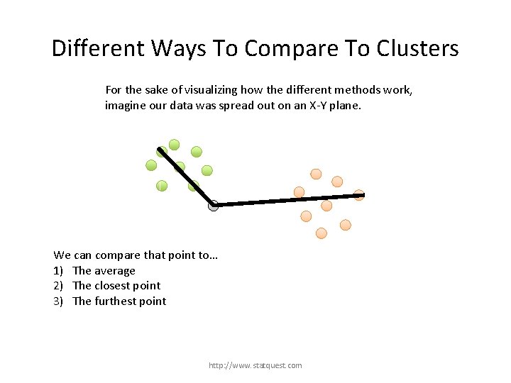
Different Ways To Compare To Clusters For the sake of visualizing how the different methods work, imagine our data was spread out on an X-Y plane. We can compare that point to… 1) The average 2) The closest point 3) The furthest point http: //www. statquest. com

Different Ways To Compare To Clusters For the sake of visualizing how the different methods work, imagine our data was spread out on an X-Y plane. We can compare that point to… 1) The average 2) The closest point 3) The furthest point 4) etc. http: //www. statquest. com

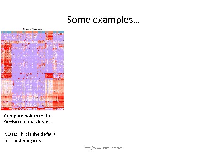
Some examples… Compare points to the furthest in the cluster. NOTE: This is the default for clustering in R. http: //www. statquest. com

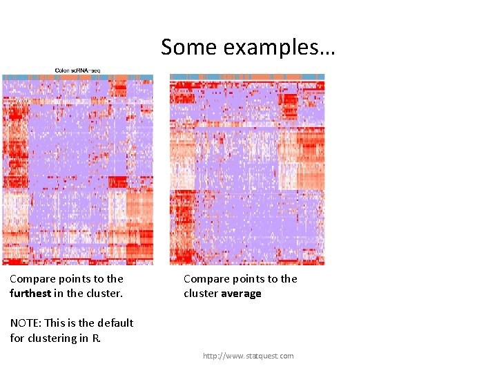
Some examples… Compare points to the furthest in the cluster. Compare points to the cluster average NOTE: This is the default for clustering in R. http: //www. statquest. com

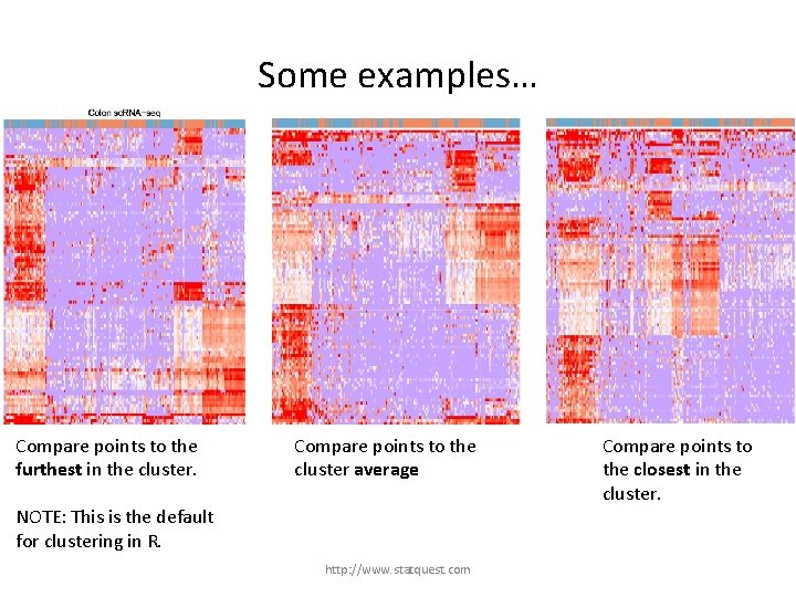
Some examples… Compare points to the furthest in the cluster. Compare points to the cluster average NOTE: This is the default for clustering in R. http: //www. statquest. com Compare points to the closest in the cluster.

In summary, to make a heatmap you: http: //www. statquest. com

In summary, to make a heatmap you: • Scale the data (either per gene, or globally). • Cluster the data (either by gene, or sample, or both gene and sample) – Hierarchical Clustering • Discussed in this Stat. Quest! – K-Means • You decide how many clusters there should be • The computer figures out which samples go in which cluster by trying to minimize some metric of dispersion (i. e. variance). http: //www. statquest. com

In summary, to make a heatmap you: • Scale the data (either per gene, per sample, or globally). • Cluster the data (either by gene, or sample, or both gene and sample) – Hierarchical Clustering • Discussed in this Stat. Quest! – K-Means • You decide how many clusters there should be • The computer figures out which samples go in which cluster by trying to minimize some metric of dispersion (i. e. variance). http: //www. statquest. com

In summary, to make a heatmap you: • Scale the data (either per gene, per sample, or globally). • Cluster the data (either by gene, or sample, or both gene and sample) – Hierarchical Clustering • Discussed in this Stat. Quest! – K-Means • You decide how many clusters there should be • The computer figures out which samples go in which cluster by trying to minimize some metric of dispersion (i. e. variance). http: //www. statquest. com

In summary, to make a heatmap you: • Scale the data (either per gene, per sample, or globally). • Cluster the data (either by gene, or sample, or both gene and sample) – Hierarchical Clustering • Discussed in this Stat. Quest! – K-Means • You decide how many clusters there should be • The computer figures out which samples go in which cluster by trying to minimize some metric of dispersion (i. e. variance). • This deserves a separate Stat. Quest!!! http: //www. statquest. com

THE END! http: //www. statquest. com