What is Clustering Also called unsupervised learning sometimes

What is Clustering? Also called unsupervised learning, sometimes called classification by statisticians and sorting by psychologists and segmentation by people in marketing • Organizing data into classes such that there is • high intra-class similarity • low inter-class similarity • Finding the class labels and the number of classes directly from the data (in contrast to classification). • More informally, finding natural groupings among objects.

What is a natural grouping among these objects?

What is a natural grouping among these objects? Clustering is subjective Simpson's Family School Employees Females Males

What is Similarity? The quality or state of being similar; likeness; resemblance; as, a similarity of features. Webster's Dictionary Similarity is hard to define, but… “We know it when we see it” The real meaning of similarity is a philosophical question. We will take a more pragmatic approach.

Defining Distance Measures Definition: Let O 1 and O 2 be two objects from the universe of possible objects. The distance (dissimilarity) between O 1 and O 2 is a real number denoted by D(O 1, O 2) Peter Piotr 0. 23 3 342. 7

Peter Piotr d('', '') = 0 d(s, '') = d('', s) = |s| -- i. e. length of s d(s 1+ch 1, s 2+ch 2) = min( d(s 1, s 2) + if ch 1=ch 2 then 0 else 1 fi, d(s 1+ch 1, s 2) + 1, d(s 1, s 2+ch 2) + 1 ) When we peek inside one of these black boxes, we see some function on two variables. These functions might very simple or very complex. In either case it is natural to ask, what properties should these functions have? 3 What properties should a distance measure have? • D(A, B) = D(B, A) • D(A, A) = 0 • D(A, B) = 0 IIf A= B • D(A, B) D(A, C) + D(B, C) Symmetry Constancy of Self-Similarity Positivity (Separation) Triangular Inequality

Intuitions behind desirable distance measure properties D(A, B) = D(B, A) Symmetry Otherwise you could claim “Alex looks like Bob, but Bob looks nothing like Alex. ” D(A, A) = 0 Constancy of Self-Similarity Otherwise you could claim “Alex looks more like Bob, than Bob does. ” D(A, B) = 0 IIf A=B Positivity (Separation) Otherwise there are objects in your world that are different, but you cannot tell apart. D(A, B) D(A, C) + D(B, C) Triangular Inequality Otherwise you could claim “Alex is very like Bob, and Alex is very like Carl, but Bob is very unlike Carl. ”

Two Types of Clustering • Partitional algorithms: Construct various partitions and then evaluate them by some criterion (we will see an example called BIRCH) • Hierarchical algorithms: Create a hierarchical decomposition of the set of objects using some criterion Hierarchical Partitional

Desirable Properties of a Clustering Algorithm • Scalability (in terms of both time and space) • Ability to deal with different data types • Minimal requirements for domain knowledge to determine input parameters • Able to deal with noise and outliers • Insensitive to order of input records • Incorporation of user-specified constraints • Interpretability and usability

A Useful Tool for Summarizing Similarity Measurements In order to better appreciate and evaluate the examples given in the early part of this talk, we will now introduce the dendrogram. The similarity between two objects in a dendrogram is represented as the height of the lowest internal node they share.

There is only one dataset that can be perfectly clustered using a hierarchy… (Bovine: 0. 69395, (Spider Monkey 0. 390, (Gibbon: 0. 36079, (Orang: 0. 33636, (Gorilla: 0. 17147, (Chimp: 0. 19268, Human: 0. 11927): 0. 08386): 0. 06124): 0. 15057): 0. 54939);

Note that hierarchies are commonly used to organize information, for example in a web portal. Yahoo’s hierarchy is manually created, we will focus on automatic creation of hierarchies in data mining. Business & Economy B 2 B Finance Aerospace Agriculture… Shopping Banking Bonds… Jobs Animals Apparel Career Workspace

A Demonstration of Hierarchical Clustering using String Edit Distance Pedro (Portuguese) Petros (Greek), Peter (English), Piotr (Polish), Peadar (Irish), Pierre (French), Peder (Danish), Peka (Hawaiian), Pietro (Italian), Piero (Italian Alternative), Petr (Czech), Pyotr (Russian) Cristovao (Portuguese) Christoph (German), Christophe (French), Cristobal (Spanish), Cristoforo (Italian), Kristoffer (Scandinavian), Krystof (Czech), Christopher (English) Miguel (Portuguese) Pie tro Ped ro Pie rre Pie ro Pet er Ped er Pek a Pea dar Mic hali Mic s hae Mig l ue Mic l k Cri stov Chr a isto o phe r Chr isto p Chr he isto ph Cri sde Cri an stob al Cri stof oro Kri stof f Kry er stof ros Pet tr Pyo Pio tr Michalis (Greek), Michael (English), Mick (Irish!)

Pedro (Portuguese/Spanish) Pio tr Pyo tr Pet ros Pie tro Ped ro Pie rre Pie ro Pet er Ped er Pek a Pea dar Petros (Greek), Peter (English), Piotr (Polish), Peadar (Irish), Pierre (French), Peder (Danish), Peka (Hawaiian), Pietro (Italian), Piero (Italian Alternative), Petr (Czech), Pyotr (Russian)

Hierarchal clustering can sometimes show patterns that are meaningless or spurious • For example, in this clustering, the tight grouping of Australia, Anguilla, St. Helena etc is meaningful, since all these countries are former UK colonies. • However the tight grouping of Niger and India is completely spurious, there is no connection between the two. AUSTRALIA St. Helena & Dependencies ANGUILLA South Georgia & South Sandwich Islands U. K. Serbia & Montenegro (Yugoslavia) FRANCE NIGER INDIA IRELAND BRAZIL

• The flag of Niger is orange over white over green, with an orange disc on the central white stripe, symbolizing the sun. The orange stands the Sahara desert, which borders Niger to the north. Green stands for the grassy plains of the south and west and for the River Niger which sustains them. It also stands for fraternity and hope. White generally symbolizes purity and hope. • The Indian flag is a horizontal tricolor in equal proportion of deep saffron on the top, white in the middle and dark green at the bottom. In the center of the white band, there is a wheel in navy blue to indicate the Dharma Chakra, the wheel of law in the Sarnath Lion Capital. This center symbol or the 'CHAKRA' is a symbol dating back to 2 nd century BC. The saffron stands for courage and sacrifice; the white, for purity and truth; the green for growth and auspiciousness. AUSTRALIA St. Helena & Dependencies ANGUILLA South Georgia & South Sandwich Islands U. K. Serbia & Montenegro (Yugoslavia) FRANCE NIGER INDIA IRELAND BRAZIL

We can look at the dendrogram to determine the “correct” number of clusters. In this case, the two highly separated subtrees are highly suggestive of two clusters. (Things are rarely this clear cut, unfortunately)

One potential use of a dendrogram is to detect outliers The single isolated branch is suggestive of a data point that is very different to all others Outlier

(How-to) Hierarchical Clustering The number of dendrograms with n leafs = (2 n -3)!/[(2(n -2)) (n -2)!] Number of Leafs 2 3 4 5. . . 10 Number of Possible Dendrograms 1 3 15 105 … 34, 459, 425 Since we cannot test all possible trees we will have to heuristic search of all possible trees. We could do this. . Bottom-Up (agglomerative): Starting with each item in its own cluster, find the best pair to merge into a new cluster. Repeat until all clusters are fused together. Top-Down (divisive): Starting with all the data in a single cluster, consider every possible way to divide the cluster into two. Choose the best division and recursively operate on both sides.

We begin with a distance matrix which contains the distances between every pair of objects in our database. 0 D( , ) = 8 D( , ) = 1 8 8 7 7 0 2 4 4 0 3 3 0 1 0

Bottom-Up (agglomerative): Starting with each item in its own cluster, find the best pair to merge into a new cluster. Repeat until all clusters are fused together. Consider all possible merges… … Choose the best

Bottom-Up (agglomerative): Starting with each item in its own cluster, find the best pair to merge into a new cluster. Repeat until all clusters are fused together. Consider all possible merges… … … Choose the best

Bottom-Up (agglomerative): Starting with each item in its own cluster, find the best pair to merge into a new cluster. Repeat until all clusters are fused together. Consider all possible merges… Choose the best … … … Choose the best

Bottom-Up (agglomerative): Starting with each item in its own cluster, find the best pair to merge into a new cluster. Repeat until all clusters are fused together. Consider all possible merges… Choose the best … … … Choose the best

We know how to measure the distance between two objects, but defining the distance between an object and a cluster, or defining the distance between two clusters is non obvious. • Single linkage (nearest neighbor): In this method the distance between two clusters is determined by the distance of the two closest objects (nearest neighbors) in the different clusters. • Complete linkage (furthest neighbor): In this method, the distances between clusters are determined by the greatest distance between any two objects in the different clusters (i. e. , by the "furthest neighbors"). • Group average linkage: linkage In this method, the distance between two clusters is calculated as the average distance between all pairs of objects in the two different clusters. • Wards Linkage: Linkage In this method, we try to minimize the variance of the merged clusters

Single linkage Average linkage Wards linkage

Summary of Hierarchal Clustering Methods • No need to specify the number of clusters in advance. • Hierarchal nature maps nicely onto human intuition for some domains • They do not scale well: time complexity of at least O(n 2), where n is the number of total objects. • Like any heuristic search algorithms, local optima are a problem. • Interpretation of results is (very) subjective.

Up to this point we have simply assumed that we can measure similarity, but How do we measure similarity? Peter Piotr 0. 23 3 342. 7

A generic technique for measuring similarity To measure the similarity between two objects, transform one of the objects into the other, and measure how much effort it took. The measure of effort becomes the distance measure. The distance between Patty and Selma. Change dress color, 1 point Change earring shape, 1 point Change hair part, 1 point D(Patty, Selma) = 3 The distance between Marge and Selma. Change dress color, Add earrings, Decrease height, Take up smoking, Lose weight, D(Marge, Selma) = 5 1 1 1 point point This is called the “edit distance” or the “transformation distance”

Edit Distance Example It is possible to transform any string Q into string C, using only Substitution, Insertion and Deletion. Assume that each of these operators has a cost associated with it. The similarity between two strings can be defined as the cost of the cheapest transformation from Q to C. How similar are the names “Peter” and “Piotr”? Assume the following cost function Substitution Insertion Deletion 1 Unit D(Peter, Piotr) is 3 Peter Note that for now we have ignored the issue of how we can find this cheapest Substitution (i for e) transformation Piter Insertion (o) er Pet Ped ro Pie rre Pie ro tro Pie ros Pet tr Pyo Pio tr Pioter Deletion (e) Piotr

Partitional Clustering • Nonhierarchical, each instance is placed in exactly one of K nonoverlapping clusters. • Since only one set of clusters is output, the user normally has to input the desired number of clusters K.

Squared Error 10 9 8 7 6 5 4 3 2 1 1 Objective Function 2 3 4 5 6 7 8 9 10

Algorithm k-means 1. Decide on a value for k. 2. Initialize the k cluster centers (randomly, if necessary). 3. Decide the class memberships of the N objects by assigning them to the nearest cluster center. 4. Re-estimate the k cluster centers, by assuming the memberships found above are correct. 5. If none of the N objects changed membership in the last iteration, exit. Otherwise goto 3.

K-means Clustering: Step 1 Algorithm: k-means, Distance Metric: Euclidean Distance 5 4 k 1 3 k 2 2 1 k 3 0 0 1 2 3 4 5

K-means Clustering: Step 2 Algorithm: k-means, Distance Metric: Euclidean Distance 5 4 k 1 3 k 2 2 1 k 3 0 0 1 2 3 4 5

K-means Clustering: Step 3 Algorithm: k-means, Distance Metric: Euclidean Distance 5 4 k 1 3 2 k 3 k 2 1 0 0 1 2 3 4 5

K-means Clustering: Step 4 Algorithm: k-means, Distance Metric: Euclidean Distance 5 4 k 1 3 2 k 3 k 2 1 0 0 1 2 3 4 5

K-means Clustering: Step 5 Algorithm: k-means, Distance Metric: Euclidean Distance k 1 k 2 k 3

Comments on the K-Means Method • Strength – Relatively efficient: O(tkn), where n is # objects, k is # clusters, and t is # iterations. Normally, k, t << n. – Often terminates at a local optimum. The global optimum may be found using techniques such as: deterministic annealing and genetic algorithms • Weakness – Applicable only when mean is defined, then what about categorical data? – Need to specify k, the number of clusters, in advance – Unable to handle noisy data and outliers – Not suitable to discover clusters with non-convex shapes

The K-Medoids Clustering Method • Find representative objects, called medoids, in clusters • PAM (Partitioning Around Medoids, 1987) – starts from an initial set of medoids and iteratively replaces one of the medoids by one of the non-medoids if it improves the total distance of the resulting clustering – PAM works effectively for small data sets, but does not scale well for large data sets

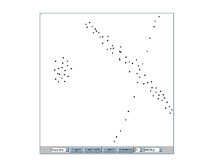
EM Algorithm • Initialize K cluster centers • Iterate between two steps – Expectation step: assign points to clusters – Maximation step: estimate model parameters

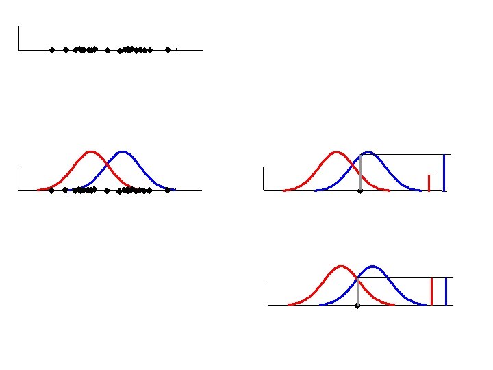
Iteration 1 The cluster means are randomly assigned

Iteration 2

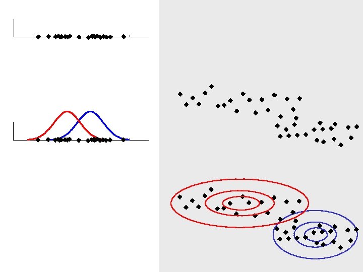
Iteration 5

Iteration 25

What happens if the data is streaming… Nearest Neighbor Clustering Not to be confused with Nearest Neighbor Classification • Items are iteratively merged into the existing clusters that are closest. • Incremental • Threshold, t, used to determine if items are added to existing clusters or a new cluster is created.

10 9 8 7 Threshold t 6 5 4 t 3 2 1 1 2 3 4 5 6 7 8 9 10

10 9 8 7 6 New data point arrives… 5 4 It is within the threshold for cluster 1, so add it to the cluster, and update cluster center. 3 2 1 1 3 2 1 2 3 4 5 6 7 8 9 10

New data point arrives… It is not within the threshold for cluster 1, so create a new cluster, and so on. . 10 4 9 8 7 6 5 4 3 2 1 1 Algorithm is highly order dependent… It is difficult to determine t in advance… 3 2 1 2 3 4 5 6 7 8 9 10

Partitional Clustering Algorithms • Clustering algorithms have been designed to handle very large datasets • E. g. the Birch algorithm • Main idea: use an in-memory R-tree to store points that are being clustered • Insert points one at a time into the R-tree, merging a new point with an existing cluster if is less than some distance away • If there are more leaf nodes than fit in memory, merge existing clusters that are close to each other • At the end of first pass we get a large number of clusters at the leaves of the R-tree § Merge clusters to reduce the number of clusters

Partitional Clustering Algorithms We need to specify the number of clusters in advance, I have chosen 2 • The Birch algorithm R 10 R 11 R 12 R 1 R 2 R 3 R 12 R 4 R 5 R 6 R 7 R 8 R 9 Data nodes containing points

Partitional Clustering Algorithms • The Birch algorithm R 10 R 11 R 12 {R 1, R 2} R 3 R 4 R 5 R 6 R 12 R 7 R 8 R 9 Data nodes containing points

Partitional Clustering Algorithms • The Birch algorithm R 10 R 11 R 12

How can we tell the right number of clusters? In general, this is a unsolved problem. However there are many approximate methods. In the next few slides we will see an example. 10 9 8 7 6 5 4 3 2 1 For our example, we will use the familiar katydid/grasshopper dataset. However, in this case we are imagining that we do NOT know the class labels. We are only clustering on the X and Y axis values. 1 2 3 4 5 6 7 8 9 10

When k = 1, the objective function is 873. 0 1 2 3 4 5 6 7 8 9 10

When k = 2, the objective function is 173. 1 1 2 3 4 5 6 7 8 9 10

When k = 3, the objective function is 133. 6 1 2 3 4 5 6 7 8 9 10

We can plot the objective function values for k equals 1 to 6… The abrupt change at k = 2, is highly suggestive of two clusters in the data. This technique for determining the number of clusters is known as “knee finding” or “elbow finding”. Objective Function 1. 00 E+03 9. 00 E+02 8. 00 E+02 7. 00 E+02 6. 00 E+02 5. 00 E+02 4. 00 E+02 3. 00 E+02 2. 00 E+02 1. 00 E+02 0. 00 E+00 1 2 3 k 4 5 6 Note that the results are not always as clear cut as in this toy example