Chapter 9 UNSUPERVISED LEARNING Clustering Part 2 Cios
- Slides: 75

Chapter 9 UNSUPERVISED LEARNING: Clustering Part 2 Cios / Pedrycz / Swiniarski / Kurgan

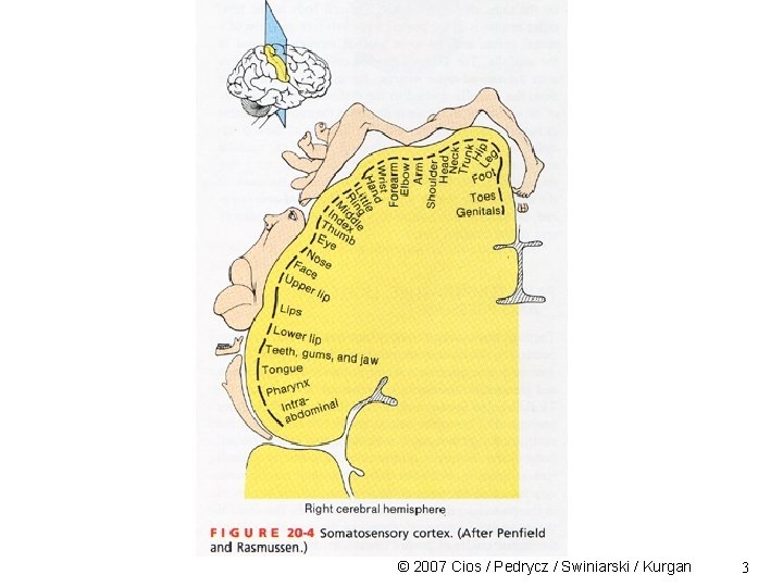
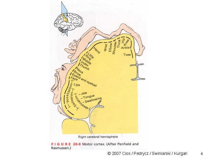
SOM Clustering Characteristics of a human associative memory: • information is retrieved/recalled on basis of some measure of similarity relating to a key pattern • memory storage and recall of “what is out there” is done via structured sequences • the recall of information from memory is dynamic © 2007 Cios / Pedrycz / Swiniarski / Kurgan 2

© 2007 Cios / Pedrycz / Swiniarski / Kurgan 3

© 2007 Cios / Pedrycz / Swiniarski / Kurgan 4

Self-Organizing Feature Maps (SOM) In data modeling it is fundamental to: • capture the topology and probability distribution of pattern vectors • map pattern vectors from the original high-D space onto the lower-D new feature space (compressed space) © 2007 Cios / Pedrycz / Swiniarski / Kurgan 5

SOM Data compression requires selection of features that best represent data for a specific purpose, e. g. , for better visual inspection of the data's structure Most attractive from the human point of view are visualizations in 2 D or 3 D space The major difficulty is how to faithfully project/map the data to ensure preservation of the topology present in the original data feature space. © 2007 Cios / Pedrycz / Swiniarski / Kurgan 6

SOM Topology-preserving properties: mapping should have these • similar patterns in the original feature space must also be similar in the reduced feature space - according to some similarity criteria • the original and the reduced space should be of "continuous nature“, i. e. , density of patterns in the reduced feature space should correspond to those in the original space. © 2007 Cios / Pedrycz / Swiniarski / Kurgan 7

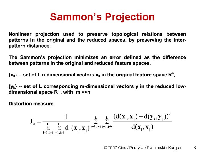
Topology-preserving Mappings Several methods were developed for topology-preserving mapping: • linear projections, such as eigenvectors • nonlinear projections, such as Sammon's projection • nonlinear projections, such as SOM neural networks © 2007 Cios / Pedrycz / Swiniarski / Kurgan 8

Sammon’s Projection © 2007 Cios / Pedrycz / Swiniarski / Kurgan 9

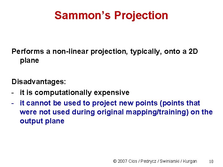
Sammon’s Projection Performs a non-linear projection, typically, onto a 2 D plane Disadvantages: - it is computationally expensive - it cannot be used to project new points (points that were not used during original mapping/training) on the output plane © 2007 Cios / Pedrycz / Swiniarski / Kurgan 10

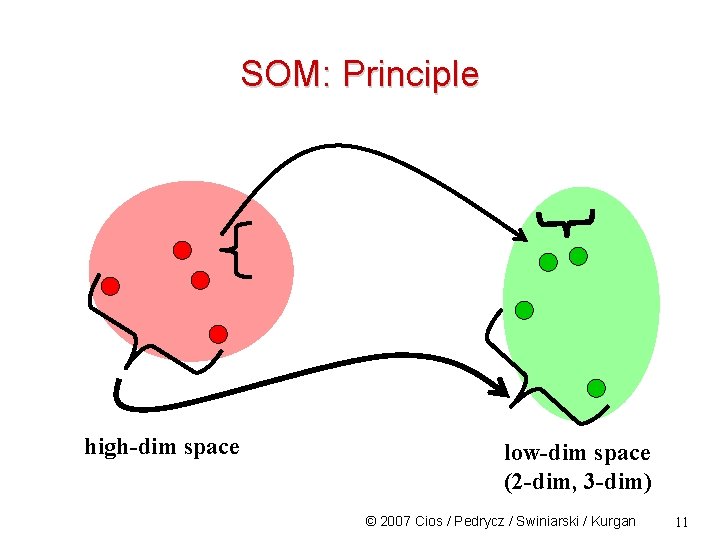
SOM: Principle high-dim space low-dim space (2 -dim, 3 -dim) © 2007 Cios / Pedrycz / Swiniarski / Kurgan 11

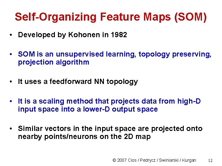
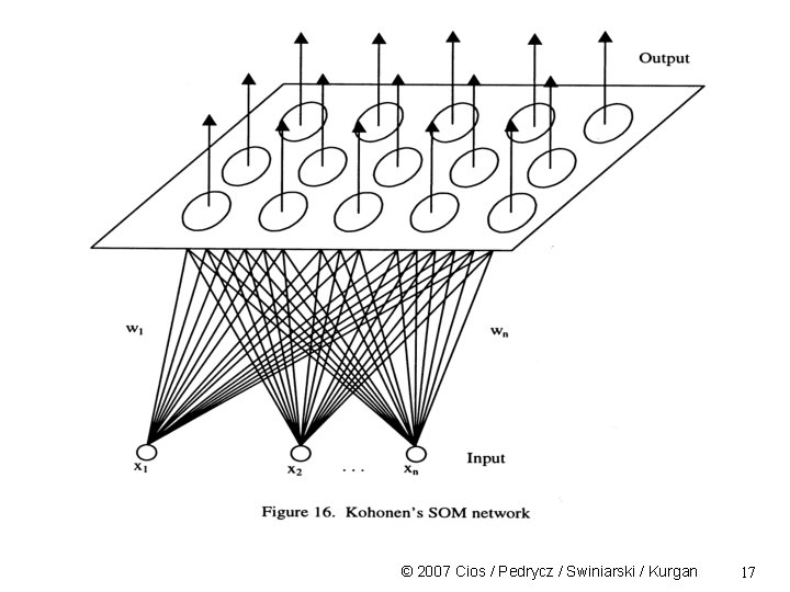
Self-Organizing Feature Maps (SOM) • Developed by Kohonen in 1982 • SOM is an unsupervised learning, topology preserving, projection algorithm • It uses a feedforward NN topology • It is a scaling method that projects data from high-D input space into a lower-D output space • Similar vectors in the input space are projected onto nearby points/neurons on the 2 D map © 2007 Cios / Pedrycz / Swiniarski / Kurgan 12

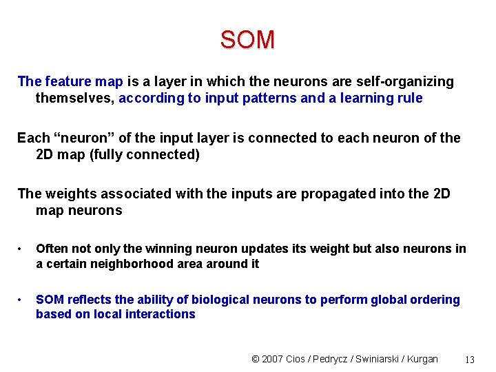
SOM The feature map is a layer in which the neurons are self-organizing themselves, according to input patterns and a learning rule Each “neuron” of the input layer is connected to each neuron of the 2 D map (fully connected) The weights associated with the inputs are propagated into the 2 D map neurons • Often not only the winning neuron updates its weight but also neurons in a certain neighborhood area around it • SOM reflects the ability of biological neurons to perform global ordering based on local interactions © 2007 Cios / Pedrycz / Swiniarski / Kurgan 13

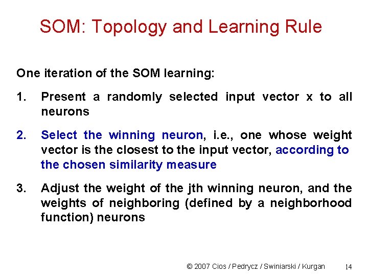
SOM: Topology and Learning Rule One iteration of the SOM learning: 1. Present a randomly selected input vector x to all neurons 2. Select the winning neuron, i. e. , one whose weight vector is the closest to the input vector, according to the chosen similarity measure 3. Adjust the weight of the jth winning neuron, and the weights of neighboring (defined by a neighborhood function) neurons © 2007 Cios / Pedrycz / Swiniarski / Kurgan 14

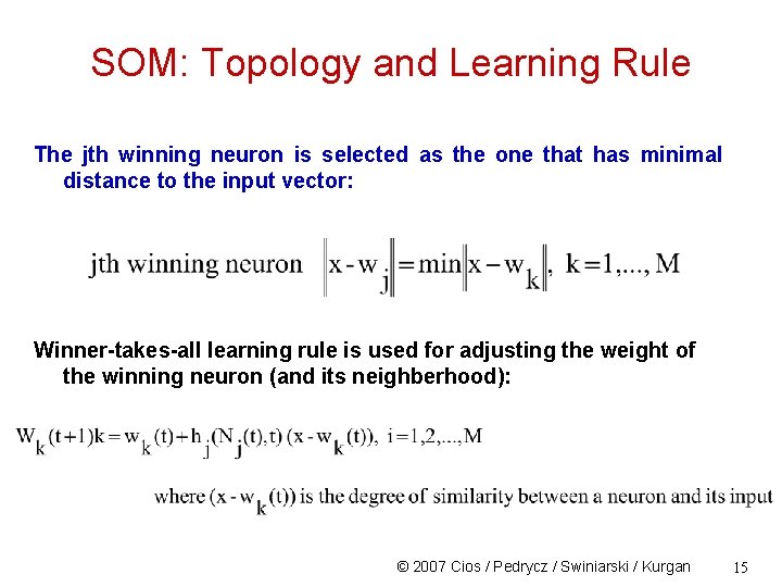
SOM: Topology and Learning Rule The jth winning neuron is selected as the one that has minimal distance to the input vector: Winner-takes-all learning rule is used for adjusting the weight of the winning neuron (and its neighberhood): © 2007 Cios / Pedrycz / Swiniarski / Kurgan 15

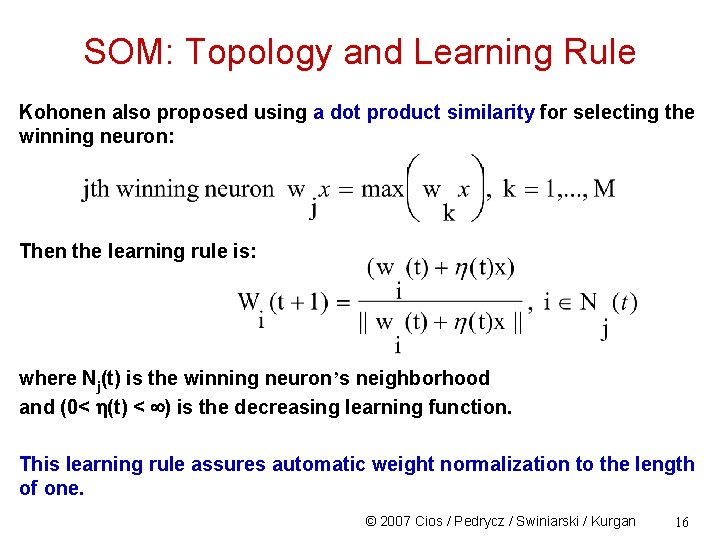
SOM: Topology and Learning Rule Kohonen also proposed using a dot product similarity for selecting the winning neuron: Then the learning rule is: where Nj(t) is the winning neuron’s neighborhood and (0< (t) < ) is the decreasing learning function. This learning rule assures automatic weight normalization to the length of one. © 2007 Cios / Pedrycz / Swiniarski / Kurgan 16

© 2007 Cios / Pedrycz / Swiniarski / Kurgan 17

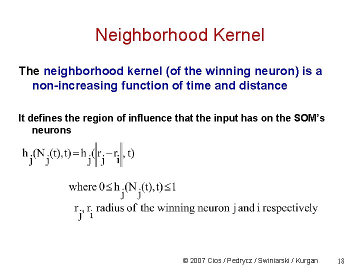
Neighborhood Kernel The neighborhood kernel (of the winning neuron) is a non-increasing function of time and distance It defines the region of influence that the input has on the SOM’s neurons © 2007 Cios / Pedrycz / Swiniarski / Kurgan 18

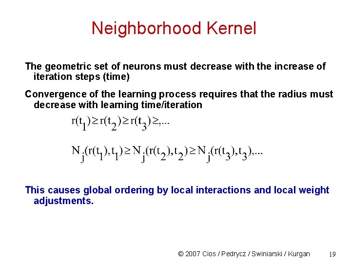
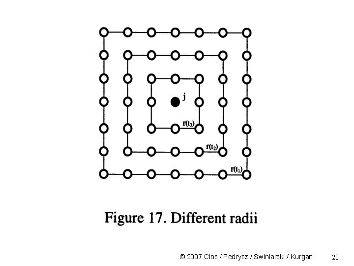
Neighborhood Kernel The geometric set of neurons must decrease with the increase of iteration steps (time) Convergence of the learning process requires that the radius must decrease with learning time/iteration This causes global ordering by local interactions and local weight adjustments. © 2007 Cios / Pedrycz / Swiniarski / Kurgan 19

© 2007 Cios / Pedrycz / Swiniarski / Kurgan 20

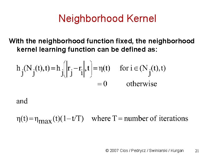
Neighborhood Kernel With the neighborhood function fixed, the neighborhood kernel learning function can be defined as: © 2007 Cios / Pedrycz / Swiniarski / Kurgan 21

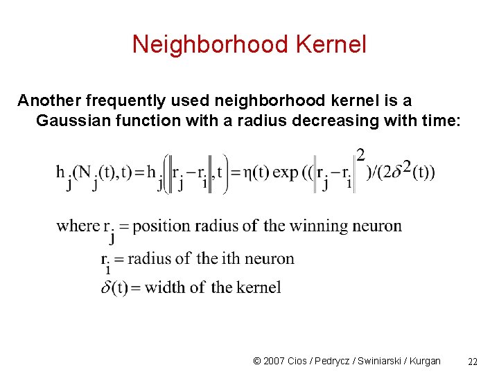
Neighborhood Kernel Another frequently used neighborhood kernel is a Gaussian function with a radius decreasing with time: © 2007 Cios / Pedrycz / Swiniarski / Kurgan 22

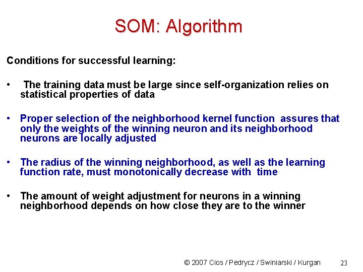
SOM: Algorithm Conditions for successful learning: • The training data must be large since self-organization relies on statistical properties of data • Proper selection of the neighborhood kernel function assures that only the weights of the winning neuron and its neighborhood neurons are locally adjusted • The radius of the winning neighborhood, as well as the learning function rate, must monotonically decrease with time • The amount of weight adjustment for neurons in a winning neighborhood depends on how close they are to the winner © 2007 Cios / Pedrycz / Swiniarski / Kurgan 23

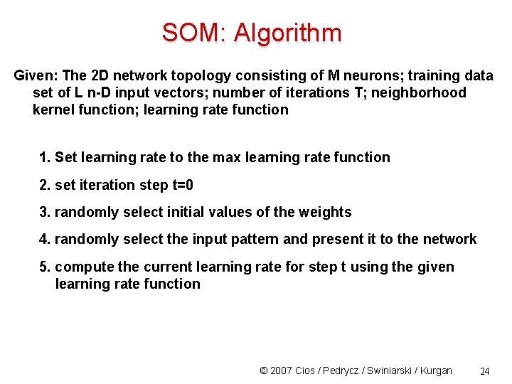
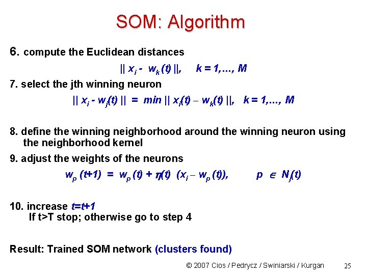
SOM: Algorithm Given: The 2 D network topology consisting of M neurons; training data set of L n-D input vectors; number of iterations T; neighborhood kernel function; learning rate function 1. Set learning rate to the max learning rate function 2. set iteration step t=0 3. randomly select initial values of the weights 4. randomly select the input pattern and present it to the network 5. compute the current learning rate for step t using the given learning rate function © 2007 Cios / Pedrycz / Swiniarski / Kurgan 24

SOM: Algorithm 6. compute the Euclidean distances || xi - wk (t) ||, k = 1, …, M 7. select the jth winning neuron || xi - wj(t) || = min || xi(t) – wk(t) ||, k = 1, …, M 8. define the winning neighborhood around the winning neuron using the neighborhood kernel 9. adjust the weights of the neurons wp (t+1) = wp (t) + (t) (xi – wp (t)), p Nj(t) 10. increase t=t+1 If t>T stop; otherwise go to step 4 Result: Trained SOM network (clusters found) © 2007 Cios / Pedrycz / Swiniarski / Kurgan 25

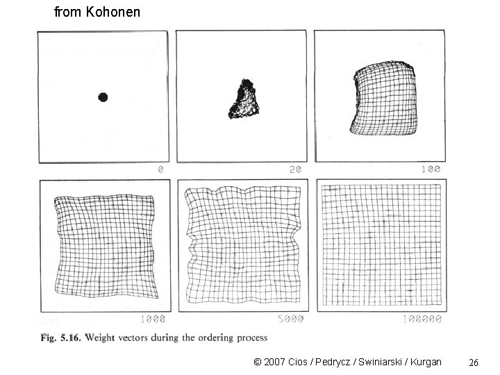
from Kohonen © 2007 Cios / Pedrycz / Swiniarski / Kurgan 26

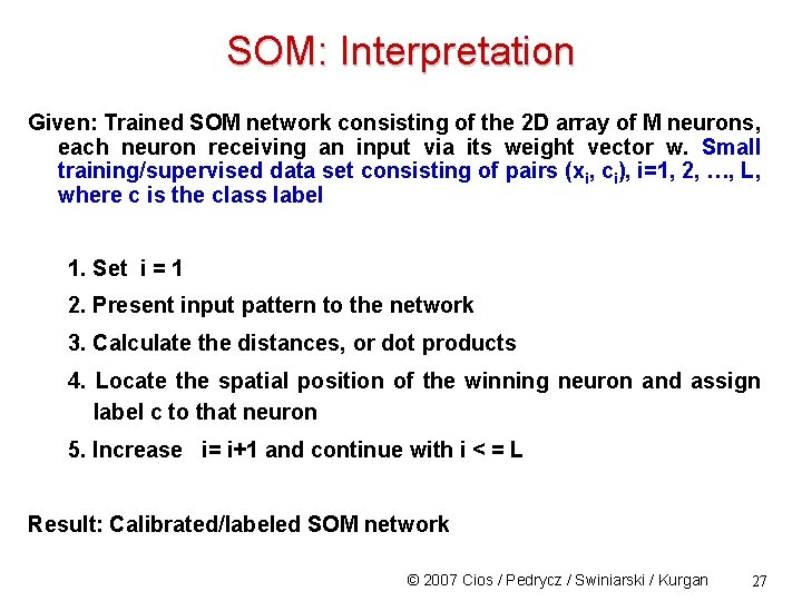
SOM: Interpretation Given: Trained SOM network consisting of the 2 D array of M neurons, each neuron receiving an input via its weight vector w. Small training/supervised data set consisting of pairs (xi, ci), i=1, 2, …, L, where c is the class label 1. Set i = 1 2. Present input pattern to the network 3. Calculate the distances, or dot products 4. Locate the spatial position of the winning neuron and assign label c to that neuron 5. Increase i= i+1 and continue with i < = L Result: Calibrated/labeled SOM network © 2007 Cios / Pedrycz / Swiniarski / Kurgan 27

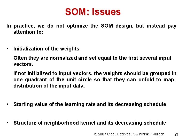
SOM: Issues In practice, we do not optimize the SOM design, but instead pay attention to: • Initialization of the weights Often they are normalized and set equal to the first several input vectors. If not initialized to input vectors, the weights should be grouped in one quadrant of the unit circle so that they can unfold to map distribution of the input data. • Starting value of the learning rate and its decreasing schedule • Structure of neighborhood kernel and its decreasing schedule © 2007 Cios / Pedrycz / Swiniarski / Kurgan 28

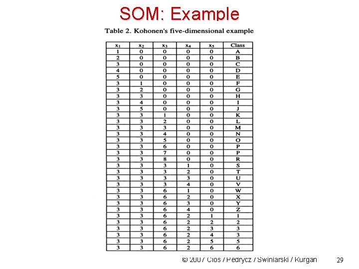
SOM: Example © 2007 Cios / Pedrycz / Swiniarski / Kurgan 29

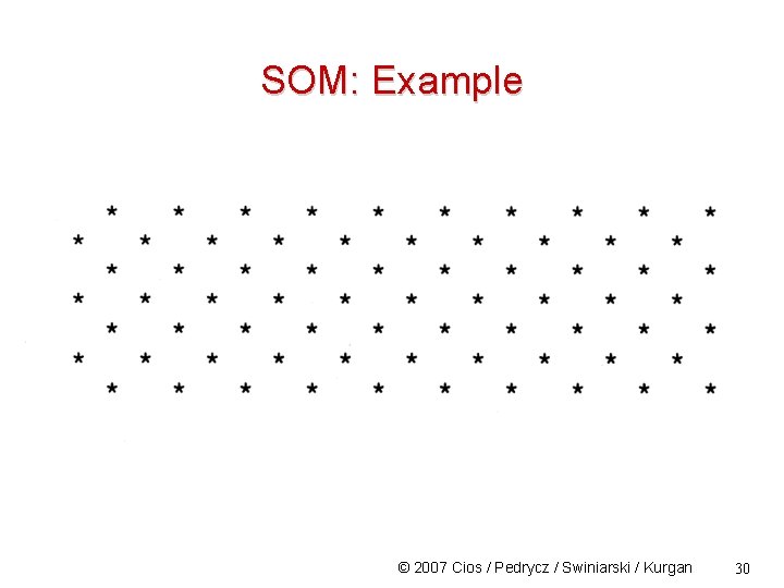
SOM: Example © 2007 Cios / Pedrycz / Swiniarski / Kurgan 30

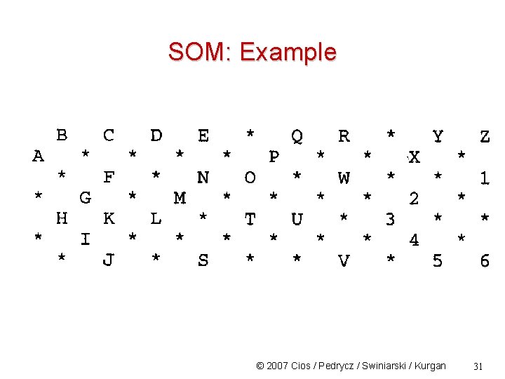
SOM: Example © 2007 Cios / Pedrycz / Swiniarski / Kurgan 31

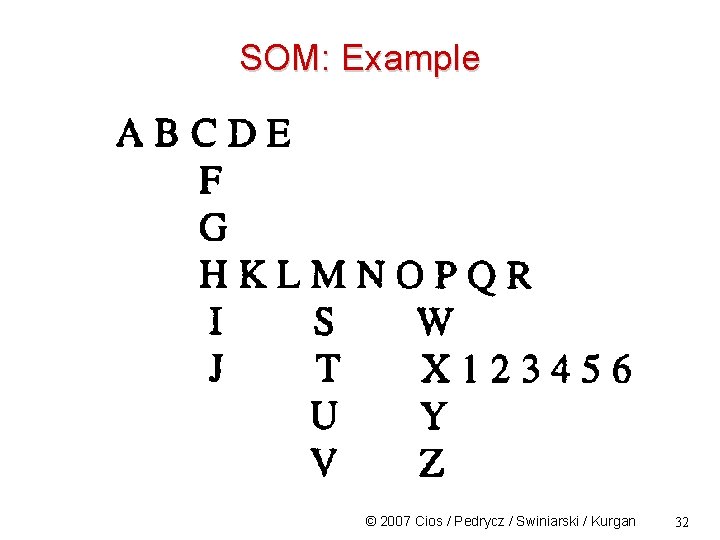
SOM: Example © 2007 Cios / Pedrycz / Swiniarski / Kurgan 32

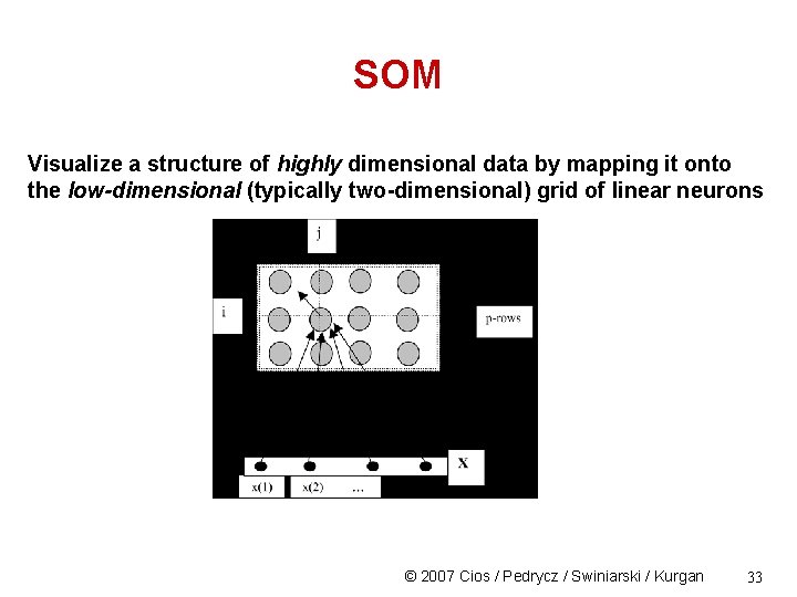
SOM Visualize a structure of highly dimensional data by mapping it onto the low-dimensional (typically two-dimensional) grid of linear neurons © 2007 Cios / Pedrycz / Swiniarski / Kurgan 33

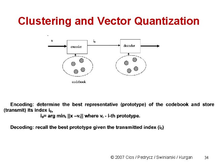
Clustering and Vector Quantization © 2007 Cios / Pedrycz / Swiniarski / Kurgan 34

Cluster validity • Using different clustering methods might result in different partitions of X, at each value of c • How many clusters truly do exist in the data? • Which clusterings are valid? • It is plausible to expect “good” clusters at more than one value of c ( 2 c < n ) © 2007 Cios / Pedrycz / Swiniarski / Kurgan 35

Aspects of Cluster Validation 1. 2. 3. 4. 5. Determine clustering tendency for a data set, i. e. , distinguish whether a non-random structure actually exists in the data. Compare results of a cluster analysis to the known class labels (if they exist). Evaluate how well the results fit the data - Use only the data Compare results of different cluster analyses results and determine “the best” one. Determining the ‘correct’ number of clusters. From : http: //www. cs. kent. edu/~jin/DM 08/Cluster. Validation. pdf 36

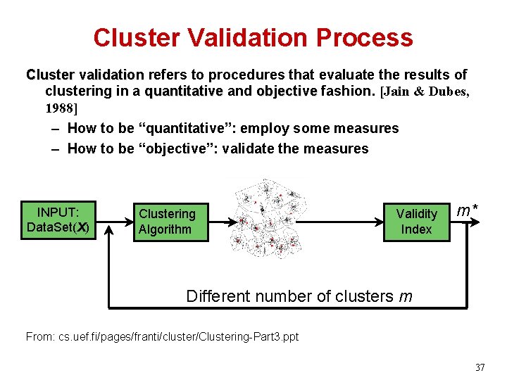
Cluster Validation Process Cluster validation refers to procedures that evaluate the results of clustering in a quantitative and objective fashion. [Jain & Dubes, 1988] – How to be “quantitative”: employ some measures – How to be “objective”: validate the measures INPUT: Data. Set(X) Clustering Algorithm Validity Index m* Different number of clusters m From: cs. uef. fi/pages/franti/cluster/Clustering-Part 3. ppt 37

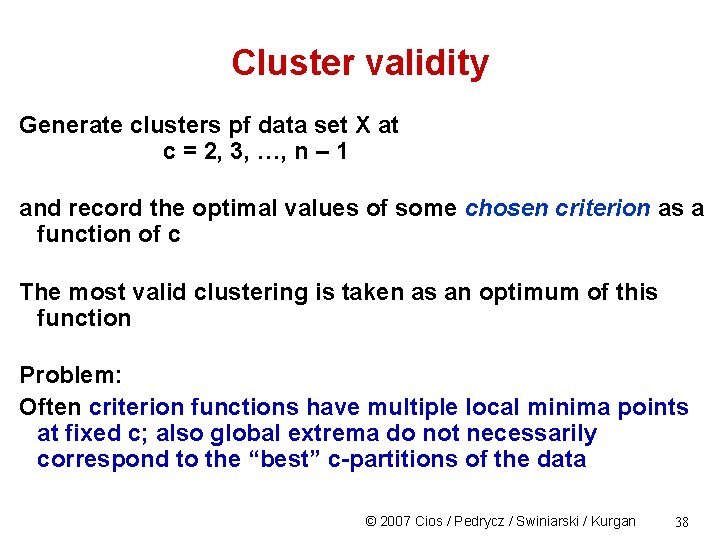
Cluster validity Generate clusters pf data set X at c = 2, 3, …, n – 1 and record the optimal values of some chosen criterion as a function of c The most valid clustering is taken as an optimum of this function Problem: Often criterion functions have multiple local minima points at fixed c; also global extrema do not necessarily correspond to the “best” c-partitions of the data © 2007 Cios / Pedrycz / Swiniarski / Kurgan 38

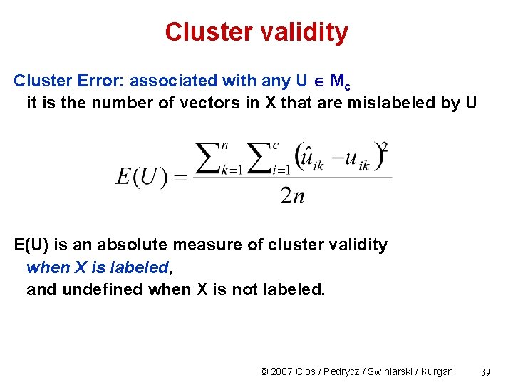
Cluster validity Cluster Error: associated with any U Mc it is the number of vectors in X that are mislabeled by U E(U) is an absolute measure of cluster validity when X is labeled, and undefined when X is not labeled. © 2007 Cios / Pedrycz / Swiniarski / Kurgan 39

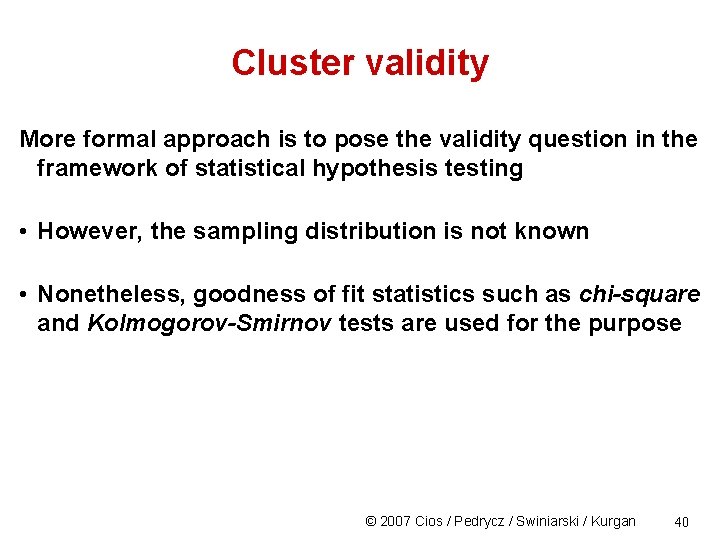
Cluster validity More formal approach is to pose the validity question in the framework of statistical hypothesis testing • However, the sampling distribution is not known • Nonetheless, goodness of fit statistics such as chi-square and Kolmogorov-Smirnov tests are used for the purpose © 2007 Cios / Pedrycz / Swiniarski / Kurgan 40

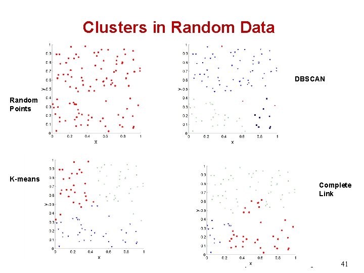
Clusters in Random Data DBSCAN Random Points K-means Complete Link © 2007 Cios / Pedrycz / Swiniarski / Kurgan 41

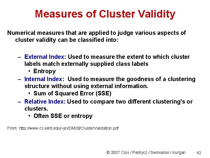
Measures of Cluster Validity Numerical measures that are applied to judge various aspects of cluster validity can be classified into: – External Index: Used to measure the extent to which cluster labels match externally supplied class labels • Entropy – Internal Index: Used to measure the goodness of a clustering structure without using external information. • Sum of Squared Error (SSE) – Relative Index: Used to compare two different clustering's or clusters. • Often SSE or entropy From: http: //www. cs. kent. edu/~jin/DM 08/Cluster. Validation. pdf © 2007 Cios / Pedrycz / Swiniarski / Kurgan 42

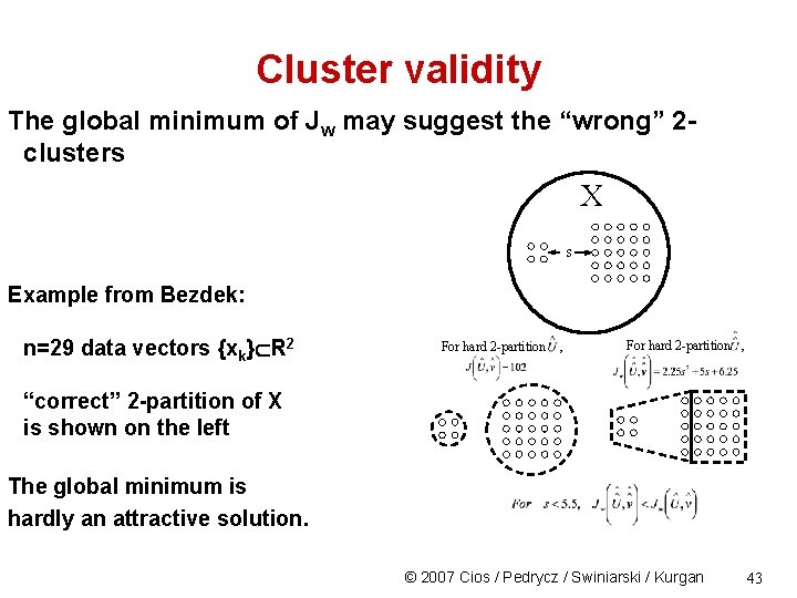
Cluster validity The global minimum of Jw may suggest the “wrong” 2 clusters X s Example from Bezdek: n=29 data vectors {xk} R 2 For hard 2 -partition , “correct” 2 -partition of X is shown on the left The global minimum is hardly an attractive solution. © 2007 Cios / Pedrycz / Swiniarski / Kurgan 43

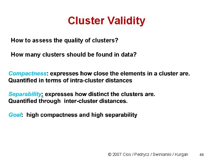
Cluster Validity How to assess the quality of clusters? How many clusters should be found in data? © 2007 Cios / Pedrycz / Swiniarski / Kurgan 44

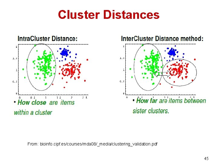
Cluster Distances From: bioinfo. cipf. es/courses/mda 08/_media/clustering_validation. pdf 45

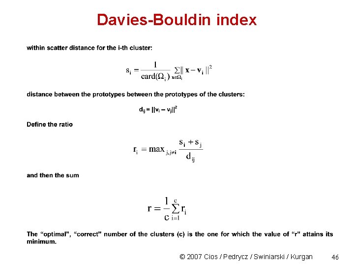
Davies-Bouldin index © 2007 Cios / Pedrycz / Swiniarski / Kurgan 46

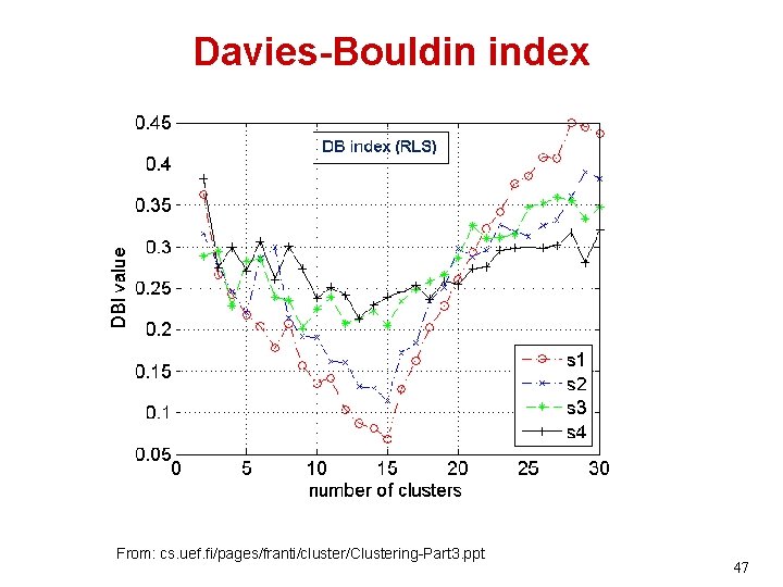
Davies-Bouldin index From: cs. uef. fi/pages/franti/cluster/Clustering-Part 3. ppt 47

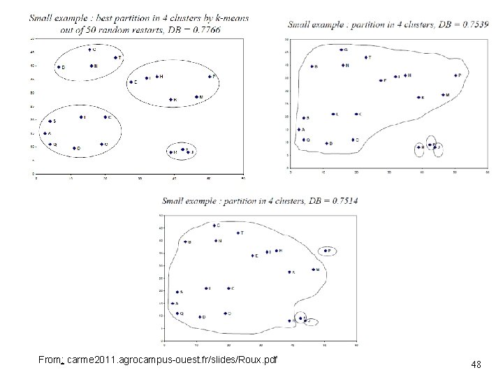
From: carme 2011. agrocampus-ouest. fr/slides/Roux. pdf 48

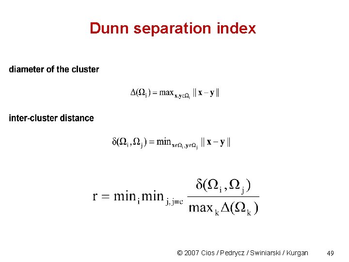
Dunn separation index © 2007 Cios / Pedrycz / Swiniarski / Kurgan 49

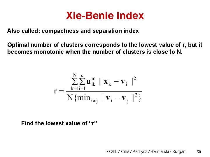
Xie-Benie index Also called: compactness and separation index Optimal number of clusters corresponds to the lowest value of r, but it becomes monotonic when the number of clusters is close to N. Find the lowest value of “r” © 2007 Cios / Pedrycz / Swiniarski / Kurgan 50

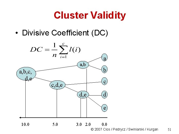
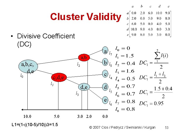
Cluster Validity • Divisive Coefficient (DC) a a, b, c, d, e b c c, d, e d e 10. 0 5. 0 3. 0 2. 0 0. 0 © 2007 Cios / Pedrycz / Swiniarski / Kurgan 51

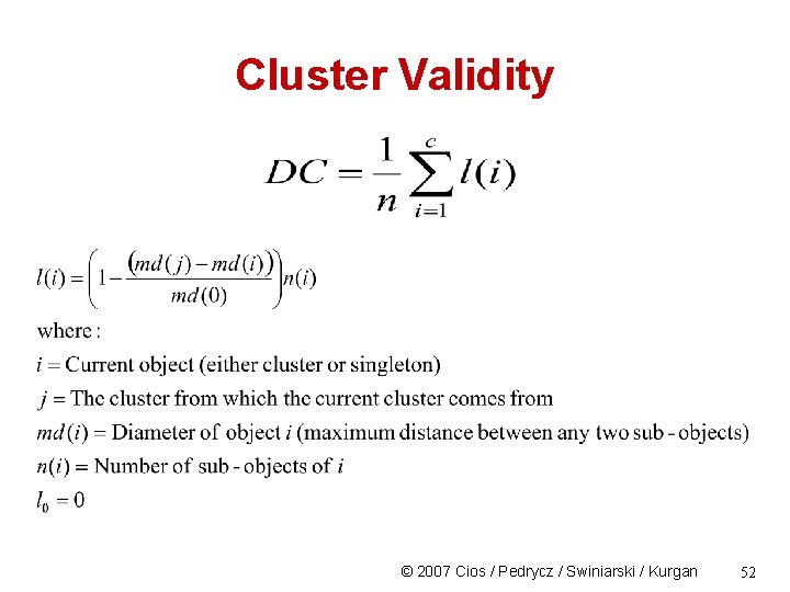
Cluster Validity © 2007 Cios / Pedrycz / Swiniarski / Kurgan 52

Cluster Validity • Divisive Coefficient (DC) a, b, c, d, e l 0 l 2 a l 7 b l 8 c c, d, e l 1 d, e d l 3 e 10. 0 5. 0 L 1=(1 -((10 -5)/10))3=1. 5 3. 0 2. 0 l 4 l 5 l 6 0. 0 © 2007 Cios / Pedrycz / Swiniarski / Kurgan 53

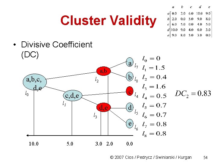
Cluster Validity • Divisive Coefficient (DC) a, b, c, d, e l 0 l 2 a l 7 b l 8 c c, d, e l 1 d, e d l 3 e 10. 0 5. 0 3. 0 2. 0 l 4 l 5 l 6 0. 0 © 2007 Cios / Pedrycz / Swiniarski / Kurgan 54

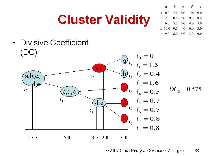
Cluster Validity • Divisive Coefficient (DC) a, b, c, d, e l 0 l 2 a l 7 b l 8 c c, d, e l 1 d, e d l 3 e 10. 0 5. 0 3. 0 2. 0 l 4 l 5 l 6 0. 0 © 2007 Cios / Pedrycz / Swiniarski / Kurgan 55

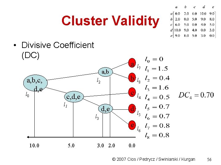
Cluster Validity • Divisive Coefficient (DC) a, b, c, d, e l 0 l 2 a l 7 b l 8 c c, d, e l 1 d, e d l 3 e 10. 0 5. 0 3. 0 2. 0 l 4 l 5 l 6 0. 0 © 2007 Cios / Pedrycz / Swiniarski / Kurgan 56

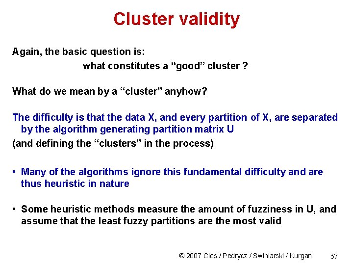
Cluster validity Again, the basic question is: what constitutes a “good” cluster ? What do we mean by a “cluster” anyhow? The difficulty is that the data X, and every partition of X, are separated by the algorithm generating partition matrix U (and defining the “clusters” in the process) • Many of the algorithms ignore this fundamental difficulty and are thus heuristic in nature • Some heuristic methods measure the amount of fuzziness in U, and assume that the least fuzzy partitions are the most valid © 2007 Cios / Pedrycz / Swiniarski / Kurgan 57

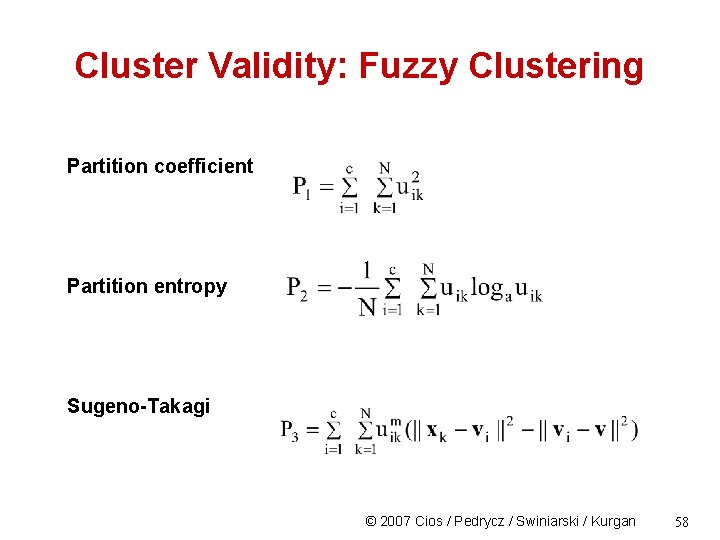
Cluster Validity: Fuzzy Clustering Partition coefficient Partition entropy Sugeno-Takagi © 2007 Cios / Pedrycz / Swiniarski / Kurgan 58

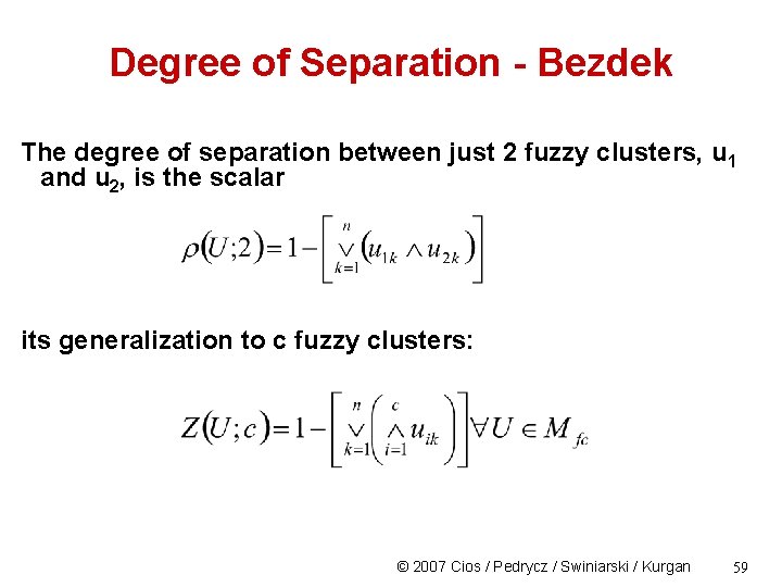
Degree of Separation - Bezdek The degree of separation between just 2 fuzzy clusters, u 1 and u 2, is the scalar its generalization to c fuzzy clusters: © 2007 Cios / Pedrycz / Swiniarski / Kurgan 59

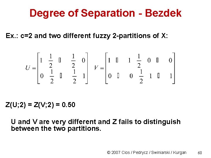
Degree of Separation - Bezdek Ex. : c=2 and two different fuzzy 2 -partitions of X: Z(U; 2) = Z(V; 2) = 0. 50 U and V are very different and Z fails to distinguish between the two partitions. © 2007 Cios / Pedrycz / Swiniarski / Kurgan 60

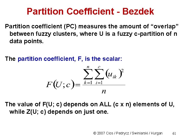
Partition Coefficient - Bezdek Partition coefficient (PC) measures the amount of “overlap” between fuzzy clusters, where U is a fuzzy c-partition of n data points. The partition coefficient, F, is the scalar: The value of F(U; c) depends on ALL (c x n) elements of U, while Z(U; c) depends on just one. © 2007 Cios / Pedrycz / Swiniarski / Kurgan 61

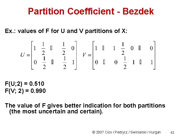
Partition Coefficient - Bezdek Ex. : values of F for U and V partitions of X: F(U; 2) = 0. 510 F(V; 2) = 0. 990 The value of F gives better indication for both partitions (the most uncertain and certain). © 2007 Cios / Pedrycz / Swiniarski / Kurgan 62

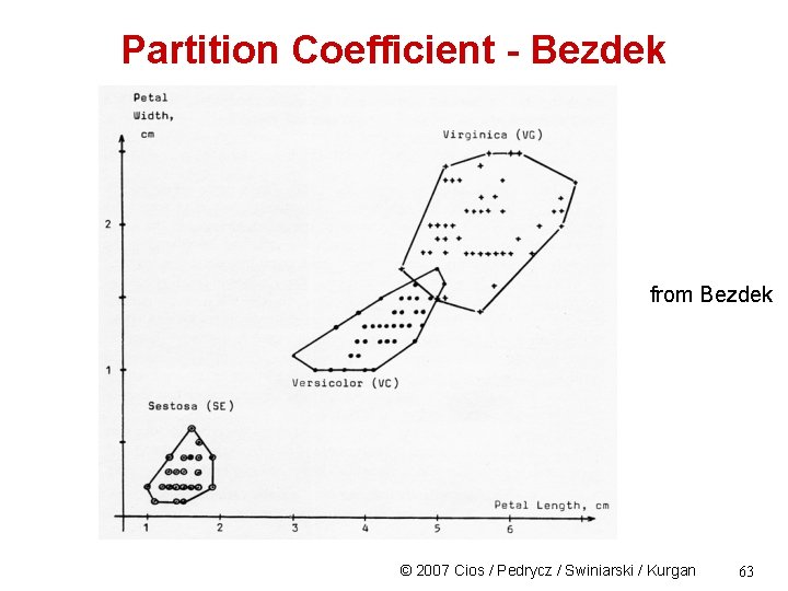
Partition Coefficient - Bezdek from Bezdek © 2007 Cios / Pedrycz / Swiniarski / Kurgan 63

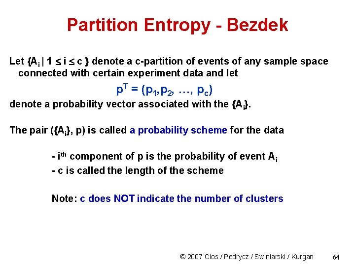
Partition Entropy - Bezdek Let {Ai | 1 i c } denote a c-partition of events of any sample space connected with certain experiment data and let p. T = (p 1, p 2, …, pc) denote a probability vector associated with the {Ai}. The pair ({Ai}, p) is called a probability scheme for the data - ith component of p is the probability of event Ai - c is called the length of the scheme Note: c does NOT indicate the number of clusters © 2007 Cios / Pedrycz / Swiniarski / Kurgan 64

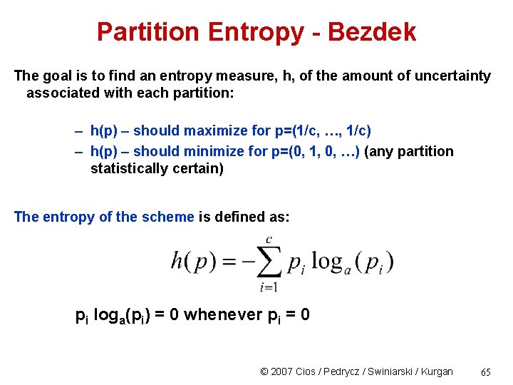
Partition Entropy - Bezdek The goal is to find an entropy measure, h, of the amount of uncertainty associated with each partition: – h(p) – should maximize for p=(1/c, …, 1/c) – h(p) – should minimize for p=(0, 1, 0, …) (any partition statistically certain) The entropy of the scheme is defined as: pi loga(pi) = 0 whenever pi = 0 © 2007 Cios / Pedrycz / Swiniarski / Kurgan 65

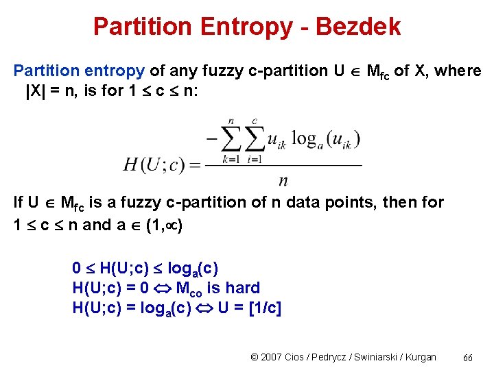
Partition Entropy - Bezdek Partition entropy of any fuzzy c-partition U Mfc of X, where |X| = n, is for 1 c n: If U Mfc is a fuzzy c-partition of n data points, then for 1 c n and a (1, ) 0 H(U; c) loga(c) H(U; c) = 0 Mco is hard H(U; c) = loga(c) U = [1/c] © 2007 Cios / Pedrycz / Swiniarski / Kurgan 66

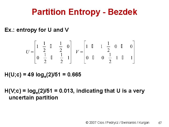
Partition Entropy - Bezdek Ex. : entropy for U and V H(U; c) = 49 loge(2)/51 = 0. 665 H(V; c) = loge(2)/51 = 0. 013, indicating that U is a very uncertain partition © 2007 Cios / Pedrycz / Swiniarski / Kurgan 67

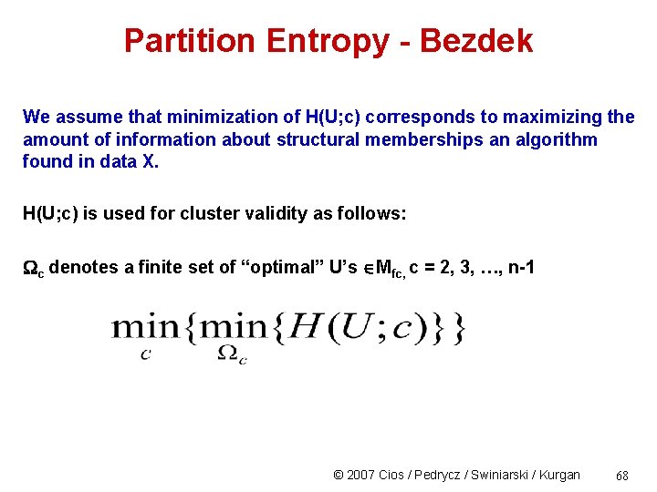
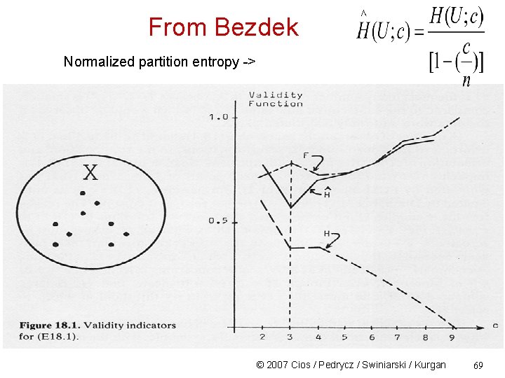
Partition Entropy - Bezdek We assume that minimization of H(U; c) corresponds to maximizing the amount of information about structural memberships an algorithm found in data X. H(U; c) is used for cluster validity as follows: c denotes a finite set of “optimal” U’s Mfc, c = 2, 3, …, n-1 © 2007 Cios / Pedrycz / Swiniarski / Kurgan 68

From Bezdek Normalized partition entropy -> © 2007 Cios / Pedrycz / Swiniarski / Kurgan 69

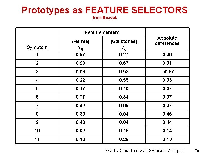
Prototypes as FEATURE SELECTORS from Bezdek Feature centers Absolute differences Symptom (Hernia) v 1 j (Gallstones) v 2 j 1 0. 57 0. 27 0. 30 2 0. 98 0. 67 0. 31 3 0. 06 0. 93 0. 87 4 0. 22 0. 55 0. 33 5 0. 17 0. 10 0. 07 6 0. 77 0. 84 0. 07 7 0. 42 0. 05 0. 37 8 0. 39 0. 84 0. 45 9 0. 48 0. 04 0. 44 10 0. 02 0. 16 0. 14 11 0. 12 0. 25 0. 13 © 2007 Cios / Pedrycz / Swiniarski / Kurgan 70

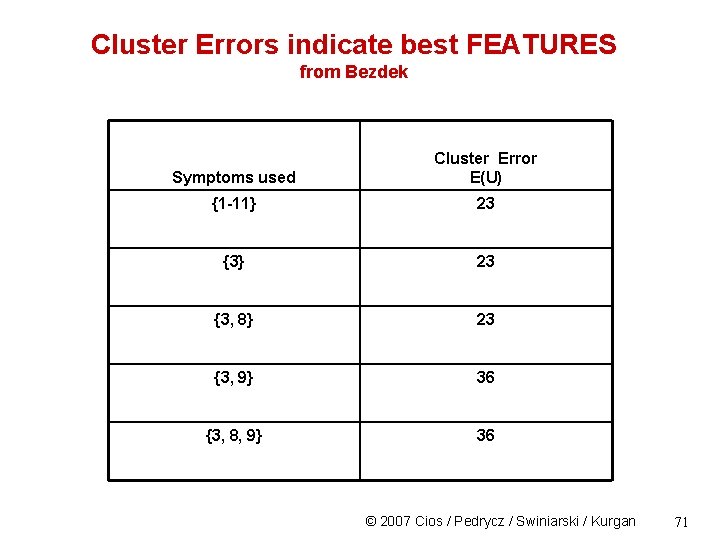
Cluster Errors indicate best FEATURES from Bezdek Symptoms used Cluster Error E(U) {1 -11} 23 {3, 8} 23 {3, 9} 36 {3, 8, 9} 36 © 2007 Cios / Pedrycz / Swiniarski / Kurgan 71

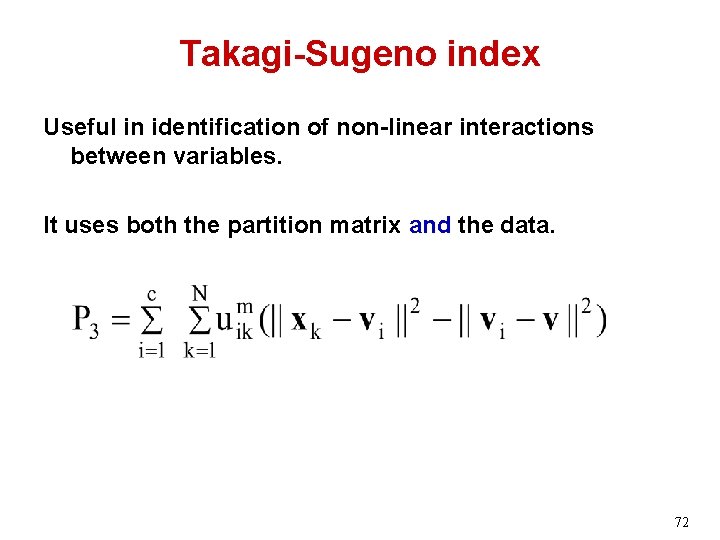
Takagi-Sugeno index Useful in identification of non-linear interactions between variables. It uses both the partition matrix and the data. 72

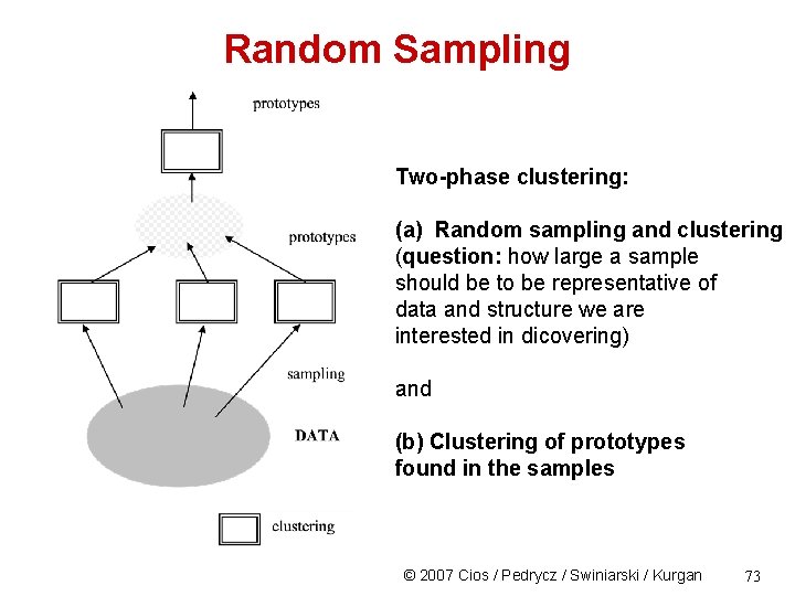
Random Sampling Two-phase clustering: (a) Random sampling and clustering (question: how large a sample should be to be representative of data and structure we are interested in dicovering) and (b) Clustering of prototypes found in the samples © 2007 Cios / Pedrycz / Swiniarski / Kurgan 73

Cluster Validity • Cluster validity is very hard to check • Without a good validation, any clustering result is potentially just a random partition of data! © 2007 Cios / Pedrycz / Swiniarski / Kurgan 74

References © 2007 Cios / Pedrycz / Swiniarski / Kurgan 75