Clustering What is Clustering Unsupervised learning Seeks to

Clustering

What is Clustering? • Unsupervised learning • Seeks to organize data into “reasonable” groups • Often based on some similarity (or distance) measure defined over data elements • Quantitative characterization may include – – – Centroid / Medoid Radius Diameter Compactness Etc.

Clustering Taxonomy • Partitional methods: – Algorithm produces a single partition or clustering of the data elements • Hierarchical methods: – Algorithm produces a series of nested partitions, each of which represents a possible clustering of the data elements • Symbolic Methods: – Algorithm produces a hierarchy of concepts

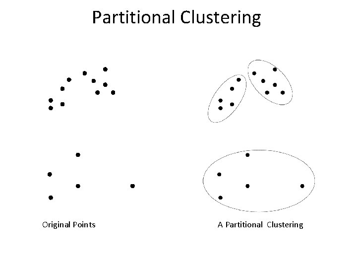
Partitional Clustering Original Points A Partitional Clustering

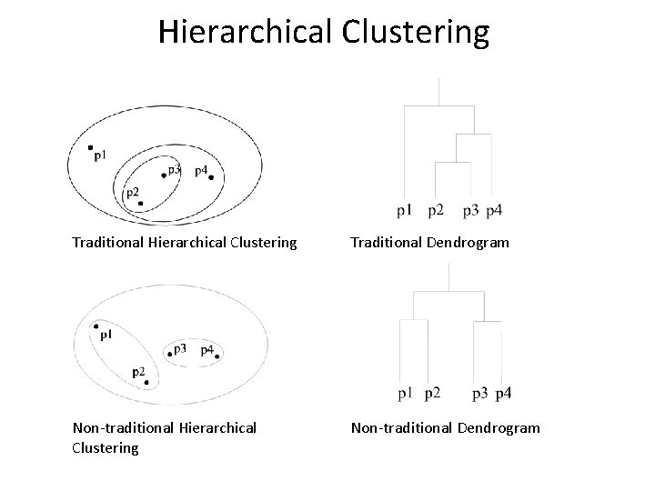
Hierarchical Clustering Traditional Dendrogram Non-traditional Hierarchical Clustering Non-traditional Dendrogram

Other Distinctions Between Sets of Clusters • Exclusive versus non-exclusive – In non-exclusive clusterings, points may belong to multiple clusters. – Can represent multiple classes or ‘border’ points • Fuzzy versus non-fuzzy – In fuzzy clustering, a point belongs to every cluster with some weight between 0 and 1 – Weights must sum to 1 – Probabilistic clustering has similar characteristics • Partial versus complete – In some cases, we only want to cluster some of the data • Heterogeneous versus homogeneous – Cluster of widely different sizes, shapes, and densities

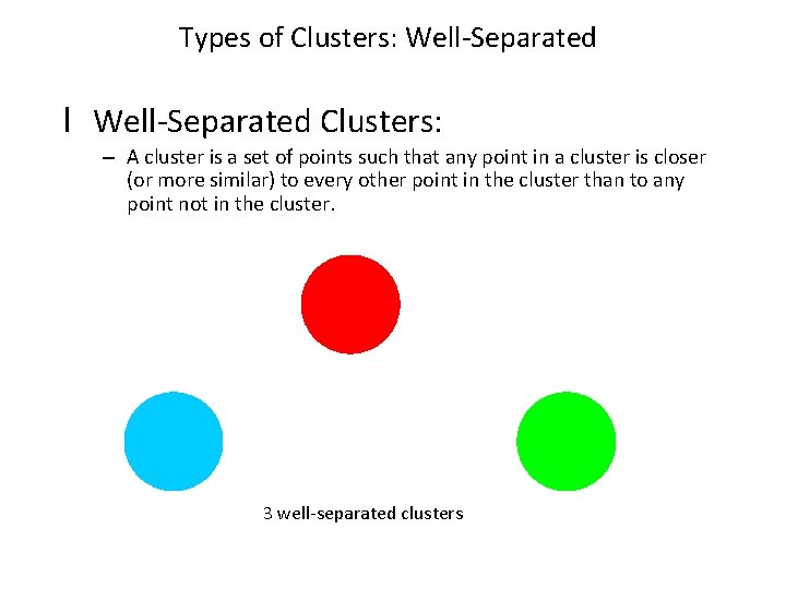
Types of Clusters: Well-Separated l Well-Separated Clusters: – A cluster is a set of points such that any point in a cluster is closer (or more similar) to every other point in the cluster than to any point not in the cluster. 3 well-separated clusters

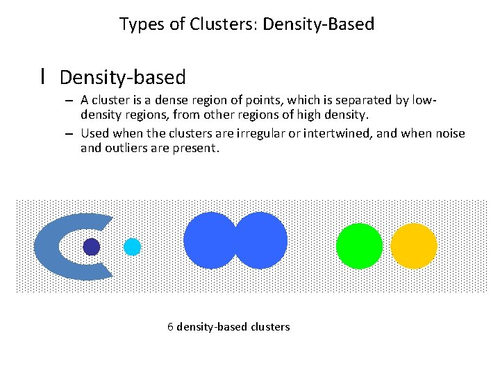
Types of Clusters: Density-Based l Density-based – A cluster is a dense region of points, which is separated by lowdensity regions, from other regions of high density. – Used when the clusters are irregular or intertwined, and when noise and outliers are present. 6 density-based clusters

Clustering Algorithms • K-means and its variants • Hierarchical clustering • Density-based clustering

Distance-based Clustering

K-means Overview • • Algorithm builds a single k-subset partition Works with numeric data only Starts with k random centroids Uses iterative re-assignment of data items to clusters based on some distance to centroids until all assignments remain unchanged

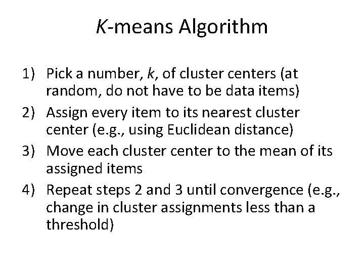
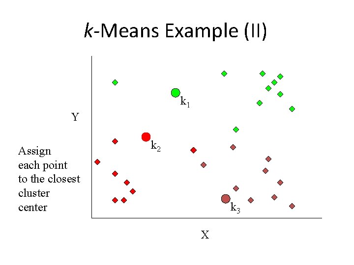
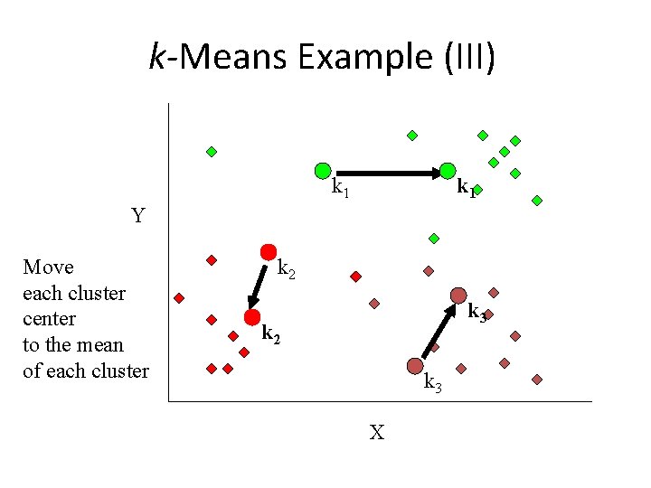
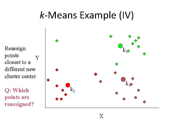
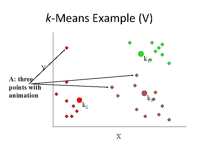
K-means Algorithm 1) Pick a number, k, of cluster centers (at random, do not have to be data items) 2) Assign every item to its nearest cluster center (e. g. , using Euclidean distance) 3) Move each cluster center to the mean of its assigned items 4) Repeat steps 2 and 3 until convergence (e. g. , change in cluster assignments less than a threshold)

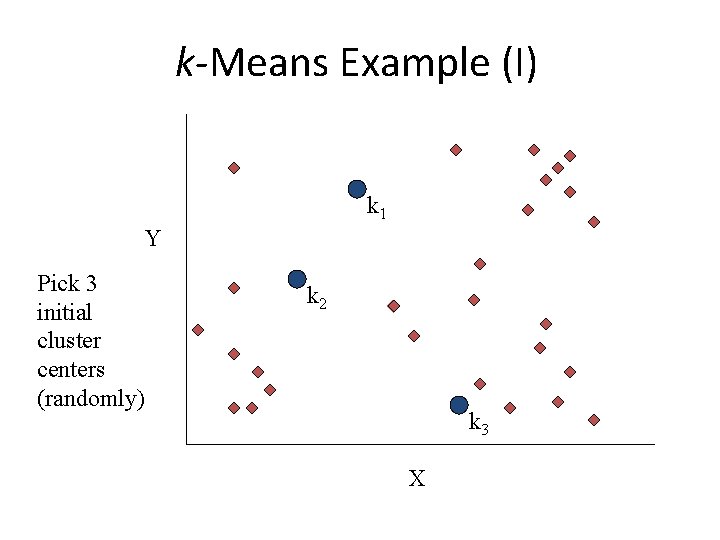
k-Means Example (I) k 1 Y Pick 3 initial cluster centers (randomly) k 2 k 3 X

k-Means Example (II) k 1 Y Assign each point to the closest cluster center k 2 k 3 X

k-Means Example (III) k 1 Y Move each cluster center to the mean of each cluster k 2 k 3 X

k-Means Example (IV) Reassign points Y closest to a different new cluster center Q: Which points are reassigned? k 1 k 3 k 2 X

k-Means Example (V) k 1 Y A: three points with animation k 3 k 2 X

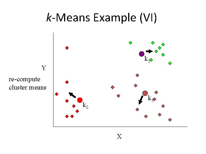
k-Means Example (VI) k 1 Y re-compute cluster means k 3 k 2 X

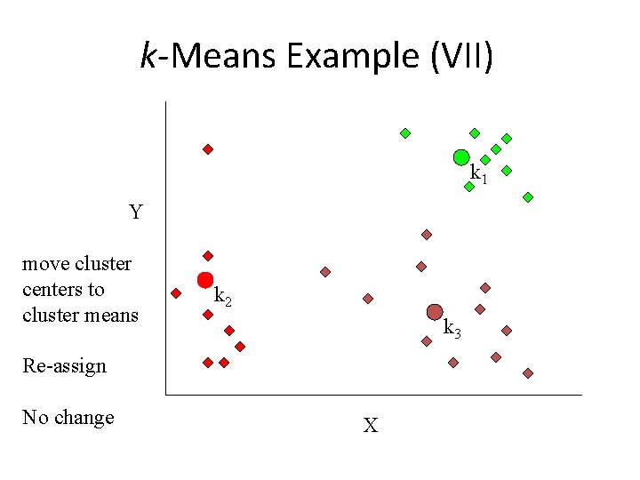
k-Means Example (VII) k 1 Y move cluster centers to cluster means k 2 k 3 Re-assign No change X

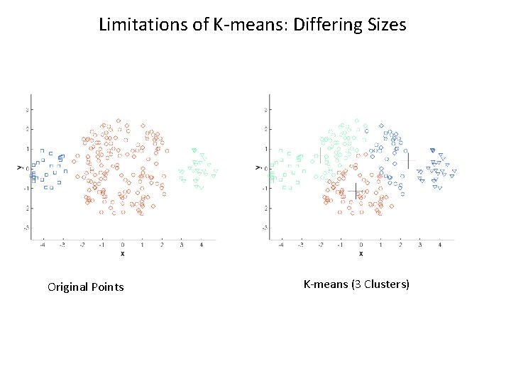
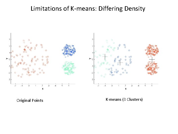
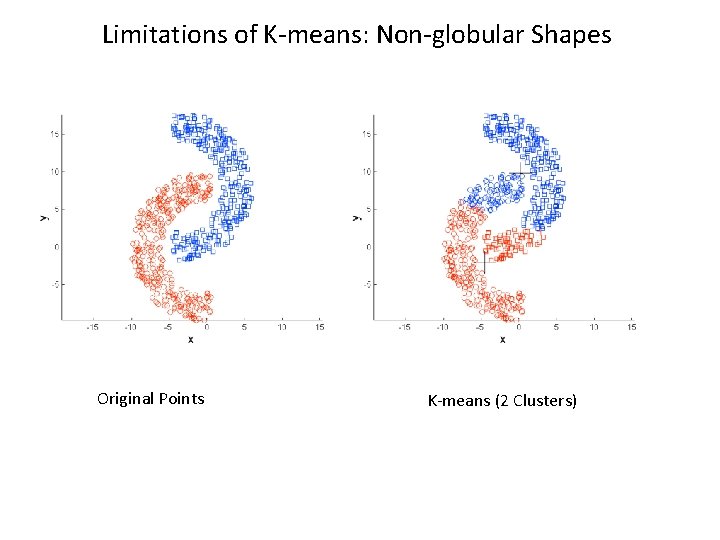
K-means Limitations • Result can vary significantly depending on initial choice of centroids • Does not handle outliers well • Has problems with clusters of different sizes, densities, or non-globular shapes • Does not scale very well

Limitations of K-means: Differing Sizes Original Points K-means (3 Clusters)

Limitations of K-means: Differing Density Original Points K-means (3 Clusters)

Limitations of K-means: Non-globular Shapes Original Points K-means (2 Clusters)

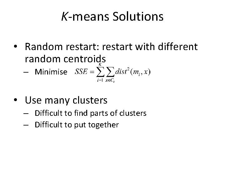
K-means Solutions • Random restart: restart with different random centroids – Minimise • Use many clusters – Difficult to find parts of clusters – Difficult to put together

K-means Summary Advantages • Simple, understandable • Items automatically assigned to clusters Disadvantages • Must pick number of clusters beforehand • All items forced into a cluster • Sensitive to outliers Time complexity is O(mkn) where m is # of iterations

K-medoids Overview • Aka Partitioning Around Medoids (PAM) • Similar to K-means: – Algorithm builds a single k-subset partition – Works with numeric data only – Uses iterative re-assignment of medoids as long as overall clustering quality improves • Difference with K-means: – Starts with k random medoids and sticks to medoids (i. e. , data points)

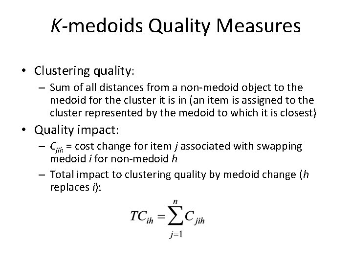
K-medoids Quality Measures • Clustering quality: – Sum of all distances from a non-medoid object to the medoid for the cluster it is in (an item is assigned to the cluster represented by the medoid to which it is closest) • Quality impact: – Cjih = cost change for item j associated with swapping medoid i for non-medoid h – Total impact to clustering quality by medoid change (h replaces i):

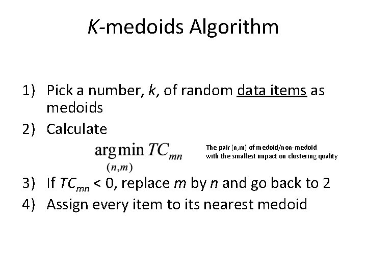
K-medoids Algorithm 1) Pick a number, k, of random data items as medoids 2) Calculate The pair (n, m) of medoid/non-medoid with the smallest impact on clustering quality 3) If TCmn < 0, replace m by n and go back to 2 4) Assign every item to its nearest medoid

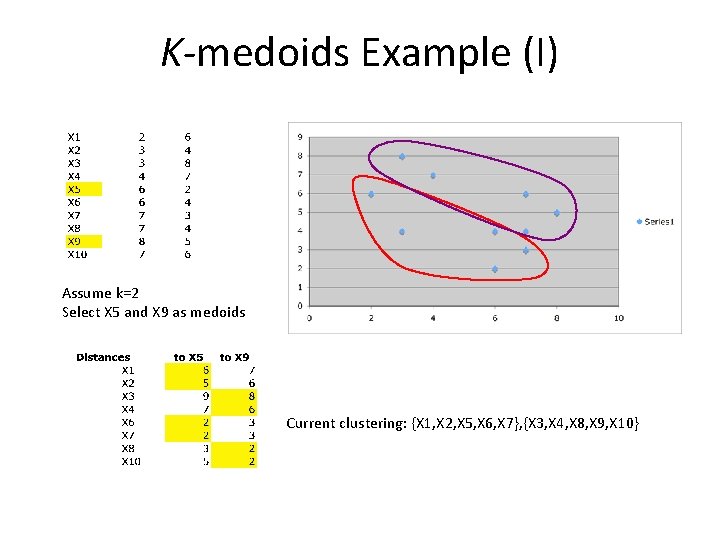
K-medoids Example (I) Assume k=2 Select X 5 and X 9 as medoids Current clustering: {X 1, X 2, X 5, X 6, X 7}, {X 3, X 4, X 8, X 9, X 10}

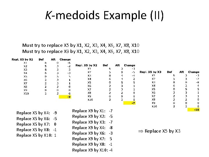
K-medoids Example (II) Must try to replace X 5 by X 1, X 2, X 3, X 4, X 6, X 7, X 8, X 10 Must try to replace X 9 by X 1, X 2, X 3, X 4, X 6, X 7, X 8, X 10 Replace X 5 by X 4: -9 Replace X 5 by X 6: -5 Replace X 5 by X 7: 0 Replace X 5 by X 8: -1 Replace X 5 by X 10: 1 Replace X 9 by X 1: -7 Replace X 9 by X 2: -5 Replace X 9 by X 3: -7 Replace X 9 by X 4: -8 Replace X 9 by X 6: -3 Replace X 9 by X 7: 5 Replace X 9 by X 8: -1 Replace X 9 by X 10: -4 Replace X 5 by X 3

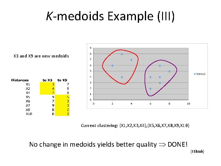
K-medoids Example (III) X 3 and X 9 are new medoids Current clustering: {X 1, X 2, X 3, X 4}, {X 5, X 6, X 7, X 8, X 9, X 10} No change in medoids yields better quality DONE! (I think)

K-medoids Discussion • As in K-means, user must select the value of k, but the resulting clustering is independent of the initial choice of medoids • Handles outliers well • Does not scale well – CLARA and CLARANS improve on the time complexity of K-medoids by using sampling and neighborhoods

K-medoids Summary Advantages • Simple, understandable • Items automatically assigned to clusters • Handles outliers Disadvantages • Must pick number of clusters beforehand • High time complexity

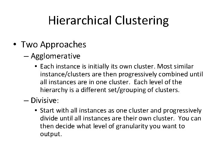
Hierarchical Clustering • Two Approaches – Agglomerative • Each instance is initially its own cluster. Most similar instance/clusters are then progressively combined until all instances are in one cluster. Each level of the hierarchy is a different set/grouping of clusters. – Divisive: • Start with all instances as one cluster and progressively divide until all instances are their own cluster. You can then decide what level of granularity you want to output.

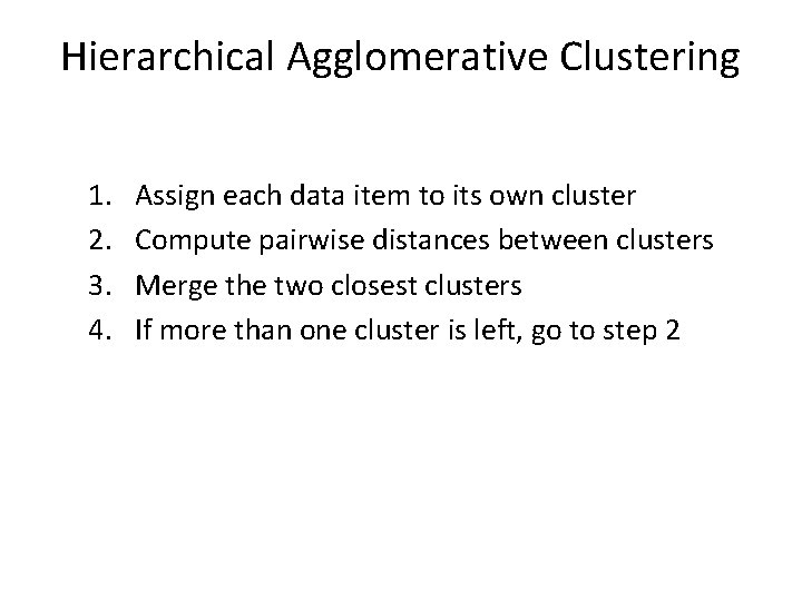
Hierarchical Agglomerative Clustering 1. 2. 3. 4. Assign each data item to its own cluster Compute pairwise distances between clusters Merge the two closest clusters If more than one cluster is left, go to step 2

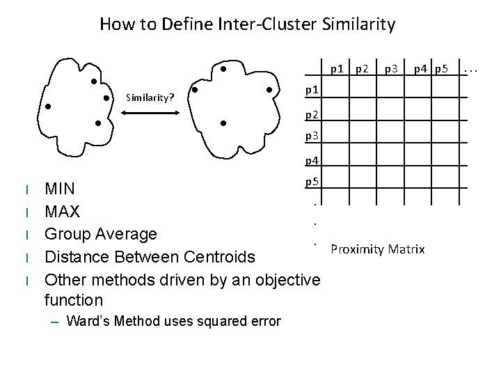
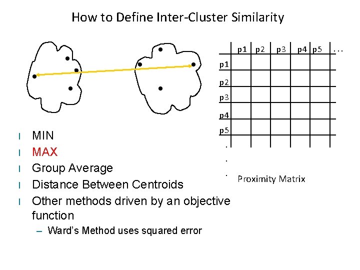
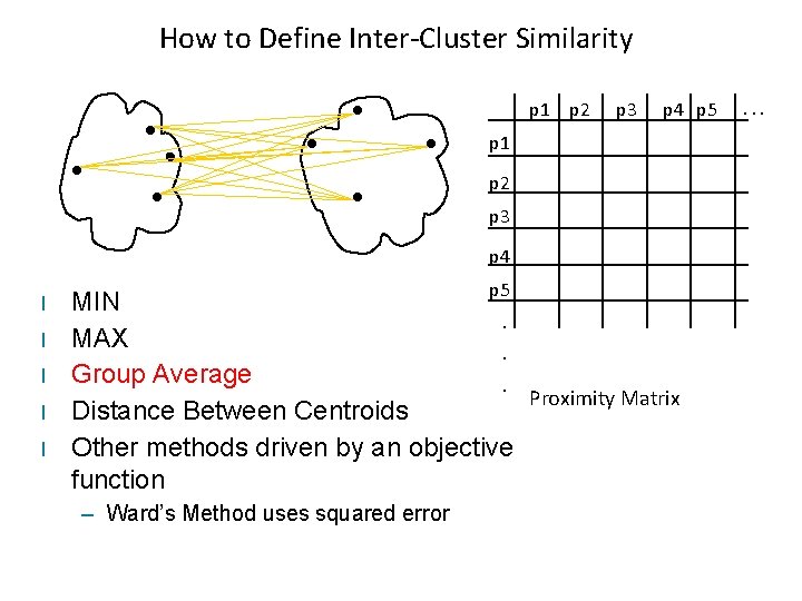
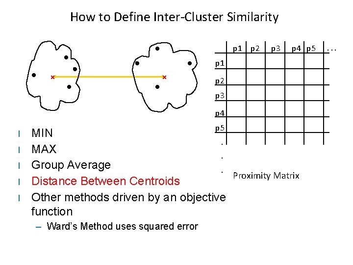
How to Define Inter-Cluster Similarity p 1 p 2 Similarity? p 3 p 4 p 5 p 1 p 2 p 3 p 4 l l l p 5 MIN. MAX. Group Average. Proximity Matrix Distance Between Centroids Other methods driven by an objective function – Ward’s Method uses squared error . . .

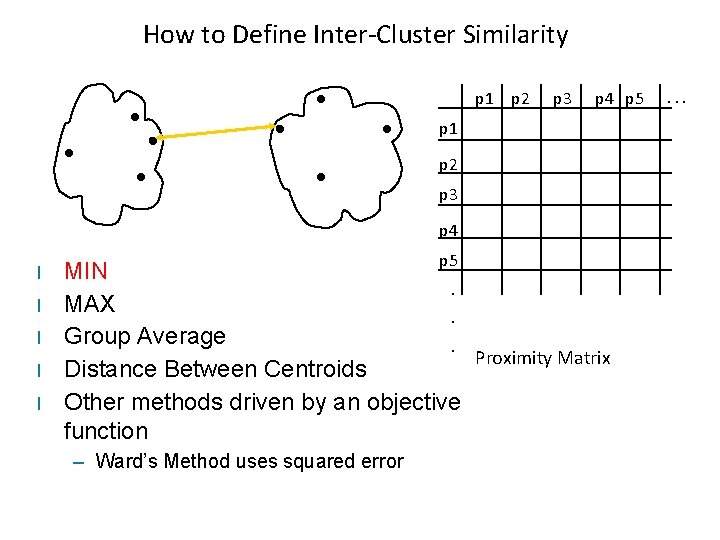
How to Define Inter-Cluster Similarity p 1 p 2 p 3 p 4 p 5 p 1 p 2 p 3 p 4 l l l p 5 MIN. MAX. Group Average. Proximity Matrix Distance Between Centroids Other methods driven by an objective function – Ward’s Method uses squared error . . .

How to Define Inter-Cluster Similarity p 1 p 2 p 3 p 4 p 5 p 1 p 2 p 3 p 4 l l l p 5 MIN. MAX. Group Average. Proximity Matrix Distance Between Centroids Other methods driven by an objective function – Ward’s Method uses squared error . . .

How to Define Inter-Cluster Similarity p 1 p 2 p 3 p 4 p 5 p 1 p 2 p 3 p 4 l l l p 5 MIN. MAX. Group Average. Proximity Matrix Distance Between Centroids Other methods driven by an objective function – Ward’s Method uses squared error . . .

How to Define Inter-Cluster Similarity p 1 p 2 p 3 p 4 p 5 p 1 p 2 p 3 p 4 l l l p 5 MIN. MAX. Group Average. Proximity Matrix Distance Between Centroids Other methods driven by an objective function – Ward’s Method uses squared error . . .

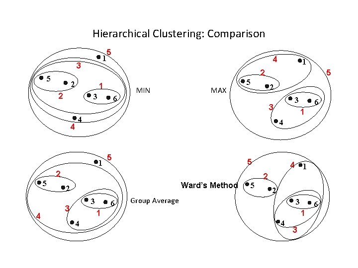
Typical Cluster Distances • Complete-link (MAX) – Maximum pairwise distance between the items of two different clusters • Single-link (MIN) – Minimum pairwise distance between the items of two different clusters • Average-link (Group Average) – Average pairwise distance between the items of two different clusters

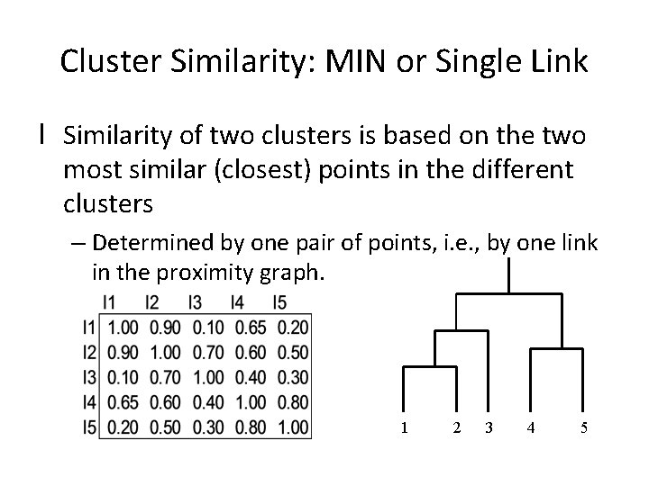
Cluster Similarity: MIN or Single Link l Similarity of two clusters is based on the two most similar (closest) points in the different clusters – Determined by one pair of points, i. e. , by one link in the proximity graph. 1 2 3 4 5

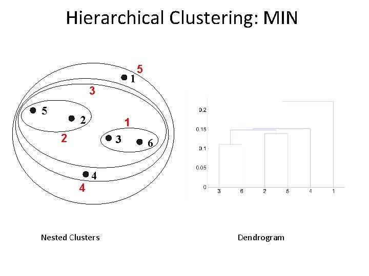
Hierarchical Clustering: MIN 1 3 5 2 1 2 3 4 5 6 4 Nested Clusters Dendrogram

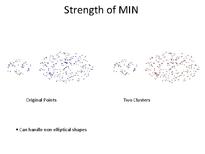
Strength of MIN Original Points • Can handle non-elliptical shapes Two Clusters

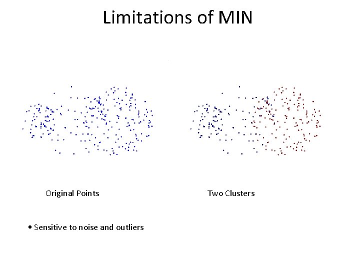
Limitations of MIN Original Points • Sensitive to noise and outliers Two Clusters

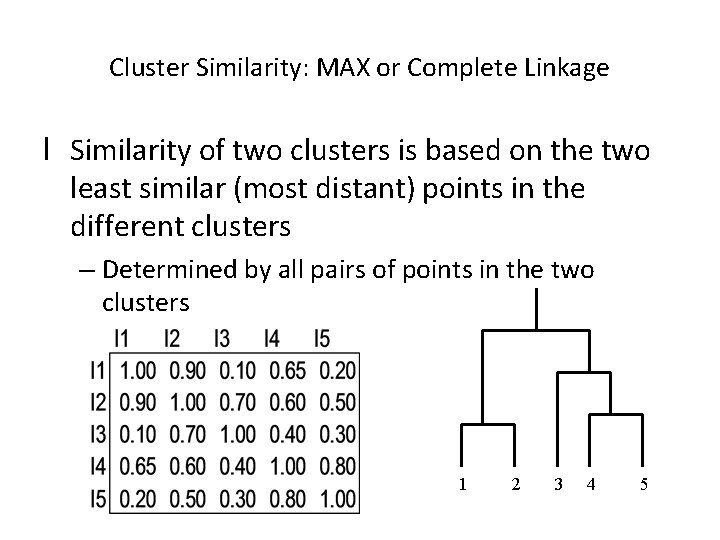
Cluster Similarity: MAX or Complete Linkage l Similarity of two clusters is based on the two least similar (most distant) points in the different clusters – Determined by all pairs of points in the two clusters 1 2 3 4 5

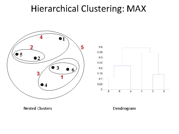
Hierarchical Clustering: MAX 4 1 5 2 3 3 6 1 4 Nested Clusters Dendrogram

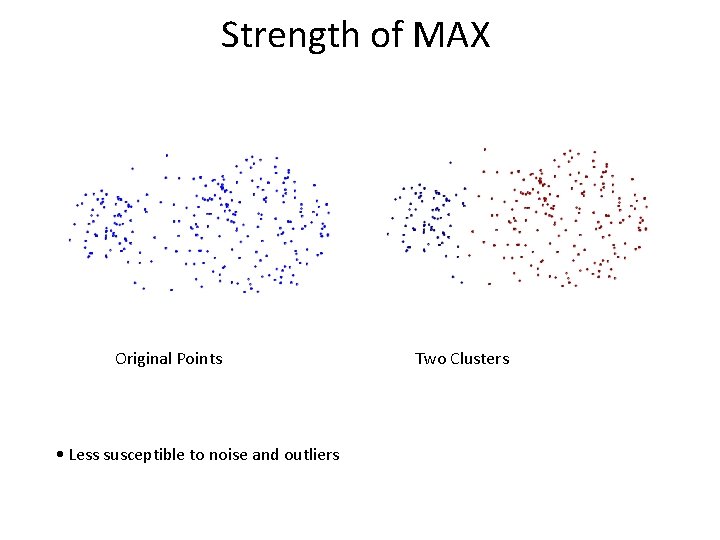
Strength of MAX Original Points • Less susceptible to noise and outliers Two Clusters

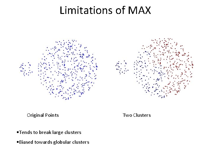
Limitations of MAX Original Points • Tends to break large clusters • Biased towards globular clusters Two Clusters

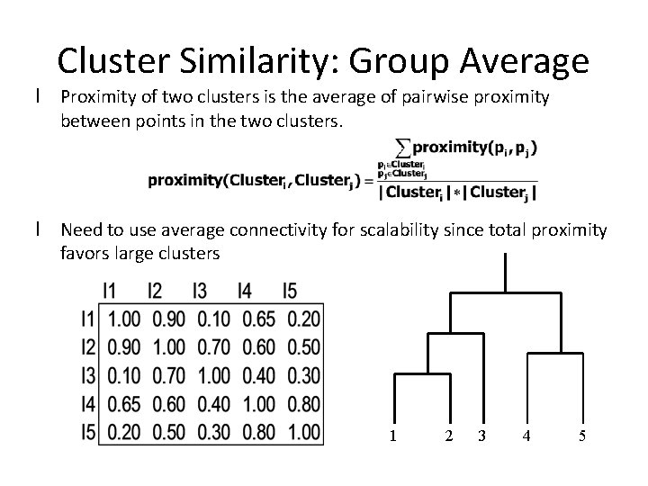
Cluster Similarity: Group Average l Proximity of two clusters is the average of pairwise proximity between points in the two clusters. l Need to use average connectivity for scalability since total proximity favors large clusters 1 2 3 4 5

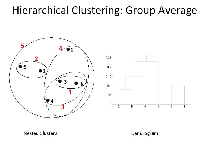
Hierarchical Clustering: Group Average 5 4 1 2 5 2 3 6 1 4 Nested Clusters 3 Dendrogram

Hierarchical Clustering: Group Average l Compromise between Single and Complete Link l Strengths – Less susceptible to noise and outliers l Limitations – Biased towards globular clusters

Cluster Similarity: Ward’s Method l Similarity of two clusters is based on the increase in squared error when two clusters are merged – Similar to group average if distance between points is distance squared l Less susceptible to noise and outliers l Biased towards globular clusters l Hierarchical analogue of K-means – Can be used to initialize K-means

Hierarchical Clustering: Comparison 1 3 5 5 1 2 3 6 MIN MAX 5 2 5 1 5 Ward’s Method 3 6 4 1 2 5 2 Group Average 3 1 4 6 4 2 3 3 3 2 4 5 4 1 5 1 2 2 4 4 6 1 4 3

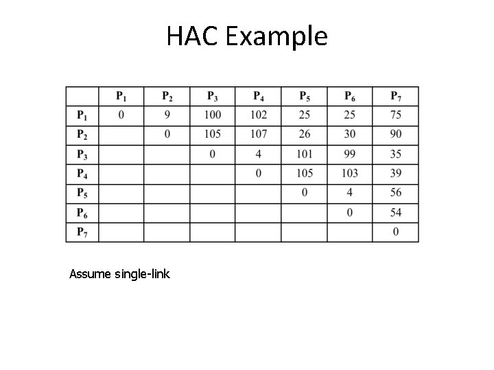
HAC Example Assume single-link

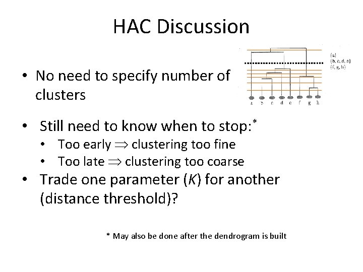
HAC Discussion • No need to specify number of clusters • Still need to know when to stop: * • Too early clustering too fine • Too late clustering too coarse • Trade one parameter (K) for another (distance threshold)? * May also be done after the dendrogram is built

Picking “the” Threshold • Guessing (sub-optimal) • Looking for “jumps” in the distance function (subjective) • Human examination (expensive, unreasonable) • Semi-supervised learning – Must-link, cannot-link constraints – Stated explicitly or implicitly (e. g. , through labels)

Simple Semi-supervised Solution Select random sample S of items Label items in S Cluster S Find the threshold value T that maximizes some clustering quality measure on S • Cluster complete dataset up to T • • |S|=50 was shown to give reasonable results

HAC Summary • Best implementation is O(n 2 logn) • All clusterings in one pass • Impact of cluster distance – Single link – can lead to long chained clusters where some points are quite far from each other – Complete link – finds more compact clusters – Average link – used less because have to recompute the average each time

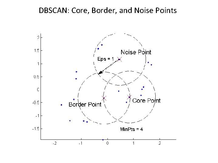
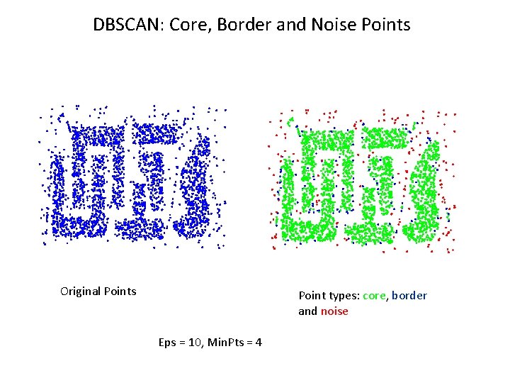
DBSCAN l DBSCAN is a density-based algorithm. – Density = number of points within a specified radius (Eps) – A point is a core point if it has more than a specified number of points (Min. Pts) within Eps // These are points that are at the interior of a cluster – A border point has fewer than Min. Pts within Eps, but is in the neighborhood of a core point – A noise point is any point that is not a core point or a border point.

DBSCAN: Core, Border, and Noise Points

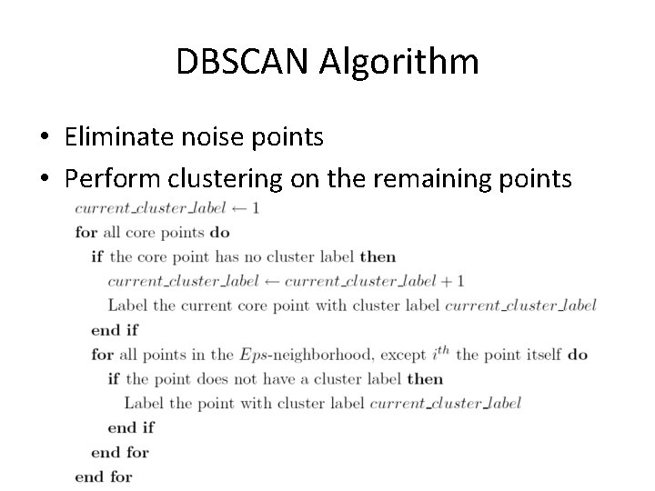
DBSCAN Algorithm • Eliminate noise points • Perform clustering on the remaining points

DBSCAN: Core, Border and Noise Points Original Points Point types: core, border and noise Eps = 10, Min. Pts = 4

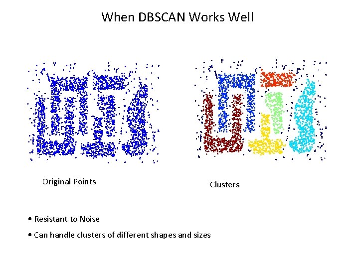
When DBSCAN Works Well Original Points Clusters • Resistant to Noise • Can handle clusters of different shapes and sizes

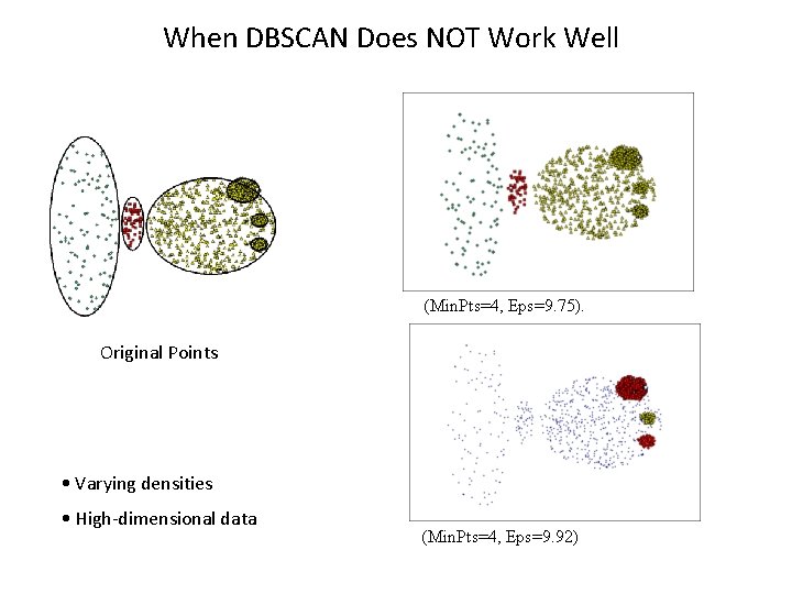
When DBSCAN Does NOT Work Well (Min. Pts=4, Eps=9. 75). Original Points • Varying densities • High-dimensional data (Min. Pts=4, Eps=9. 92)

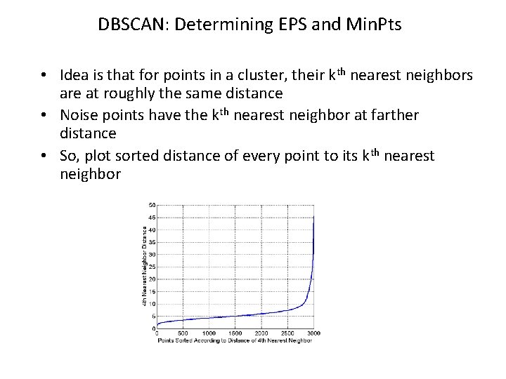
DBSCAN: Determining EPS and Min. Pts • Idea is that for points in a cluster, their kth nearest neighbors are at roughly the same distance • Noise points have the kth nearest neighbor at farther distance • So, plot sorted distance of every point to its kth nearest neighbor

Clustering Evaluation

Quality Metrics • External metrics – Computed from a comparison to actual clustering (or classification) labels. • Internal metrics – Computed solely from the composition of a cluster, with no recourse to external information.

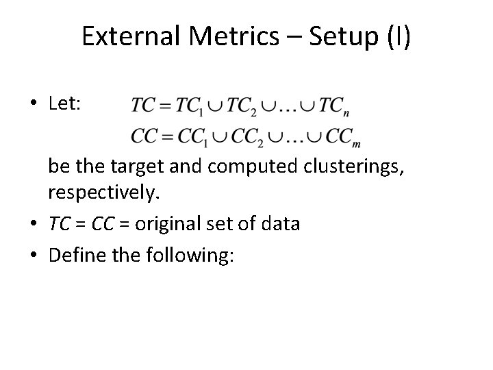
External Metrics – Setup (I) • Let: be the target and computed clusterings, respectively. • TC = CC = original set of data • Define the following:

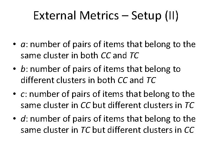
External Metrics – Setup (II) • a: number of pairs of items that belong to the same cluster in both CC and TC • b: number of pairs of items that belong to different clusters in both CC and TC • c: number of pairs of items that belong to the same cluster in CC but different clusters in TC • d: number of pairs of items that belong to the same cluster in TC but different clusters in CC

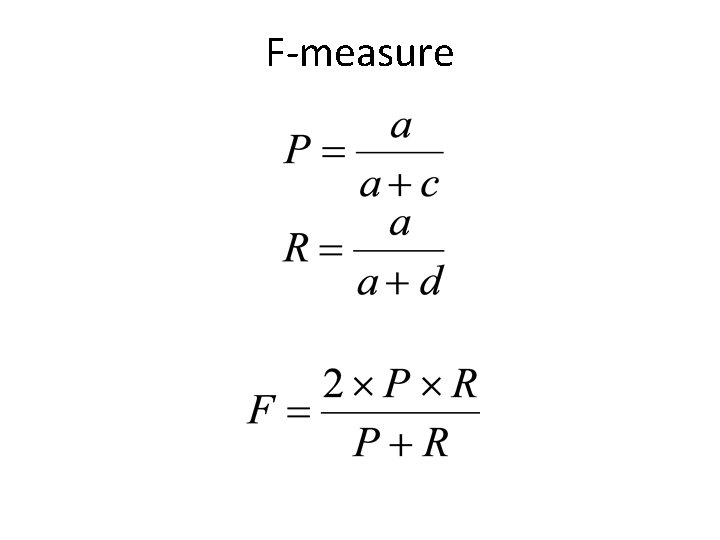
F-measure

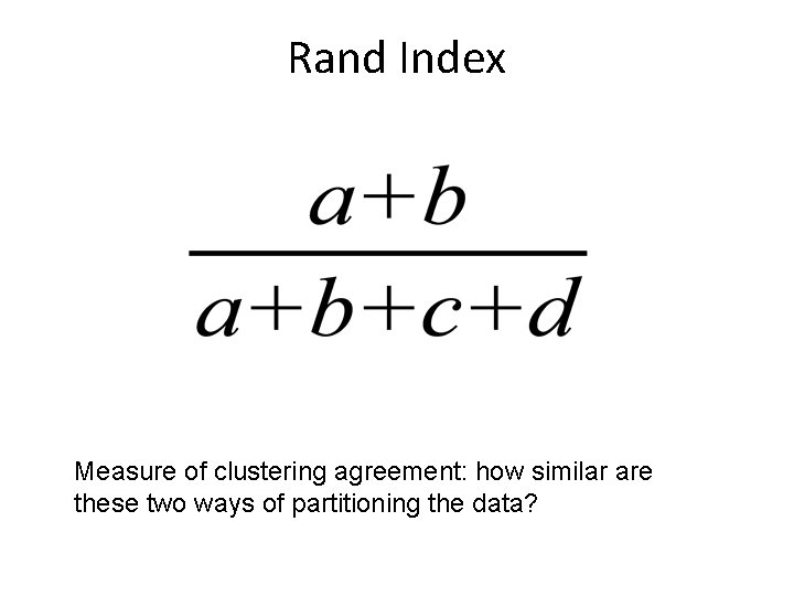
Rand Index Measure of clustering agreement: how similar are these two ways of partitioning the data?

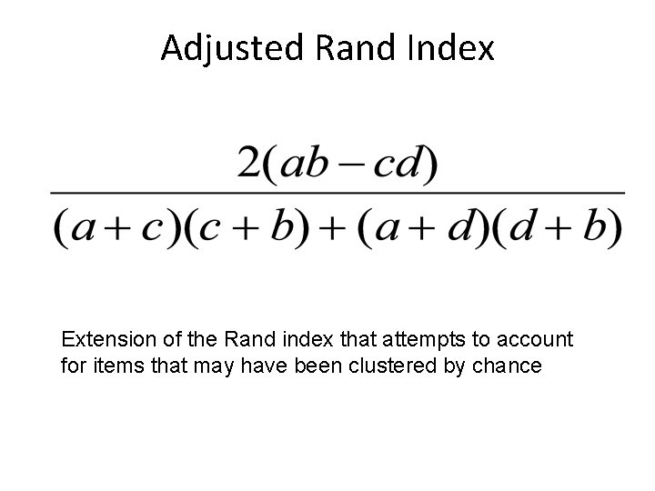
Adjusted Rand Index Extension of the Rand index that attempts to account for items that may have been clustered by chance

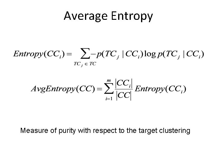
Average Entropy Measure of purity with respect to the target clustering

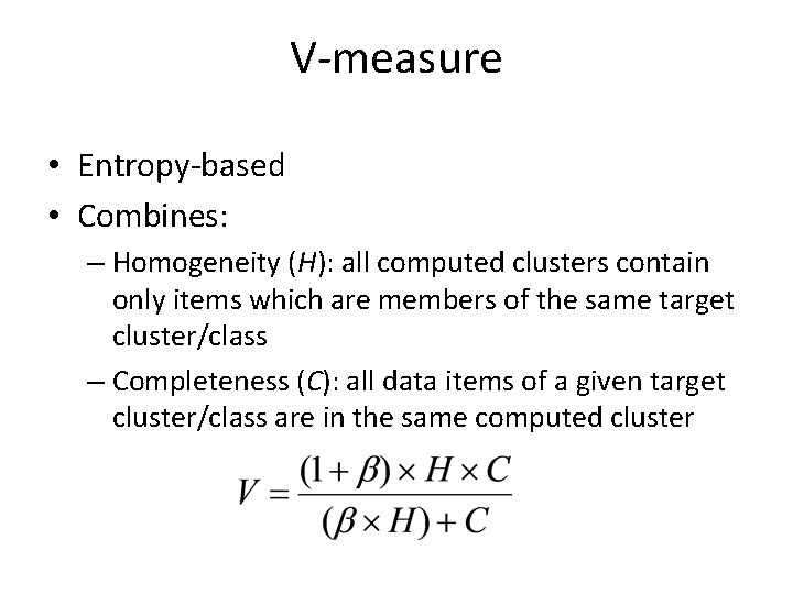
V-measure • Entropy-based • Combines: – Homogeneity (H): all computed clusters contain only items which are members of the same target cluster/class – Completeness (C): all data items of a given target cluster/class are in the same computed cluster

Internal Metrics • Assume no target clustering • Attempt to capture some intrinsic properties of the clustering – Distance-based • Sum of squares • Diameter sum or maximum • Sum of minimum distance between clusters, etc. – Probability-based • E. g. , KL divergence Just a sample presented here

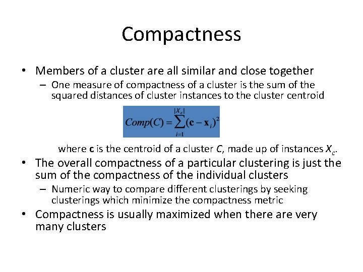
Compactness • Members of a cluster are all similar and close together – One measure of compactness of a cluster is the sum of the squared distances of cluster instances to the cluster centroid where c is the centroid of a cluster C, made up of instances Xc. • The overall compactness of a particular clustering is just the sum of the compactness of the individual clusters – Numeric way to compare different clusterings by seeking clusterings which minimize the compactness metric • Compactness is usually maximized when there are very many clusters

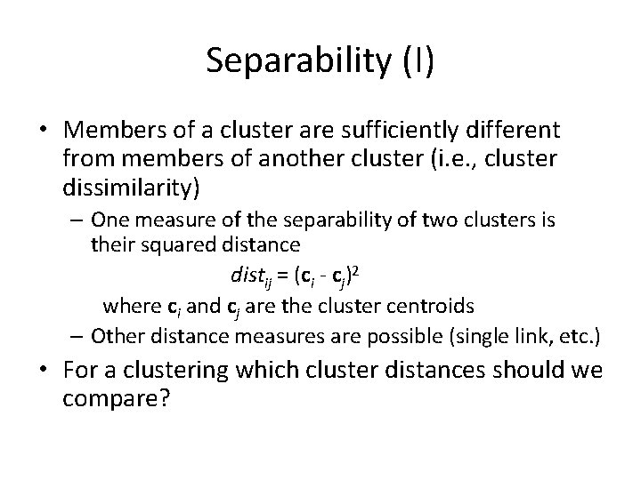
Separability (I) • Members of a cluster are sufficiently different from members of another cluster (i. e. , cluster dissimilarity) – One measure of the separability of two clusters is their squared distance distij = (ci - cj)2 where ci and cj are the cluster centroids – Other distance measures are possible (single link, etc. ) • For a clustering which cluster distances should we compare?

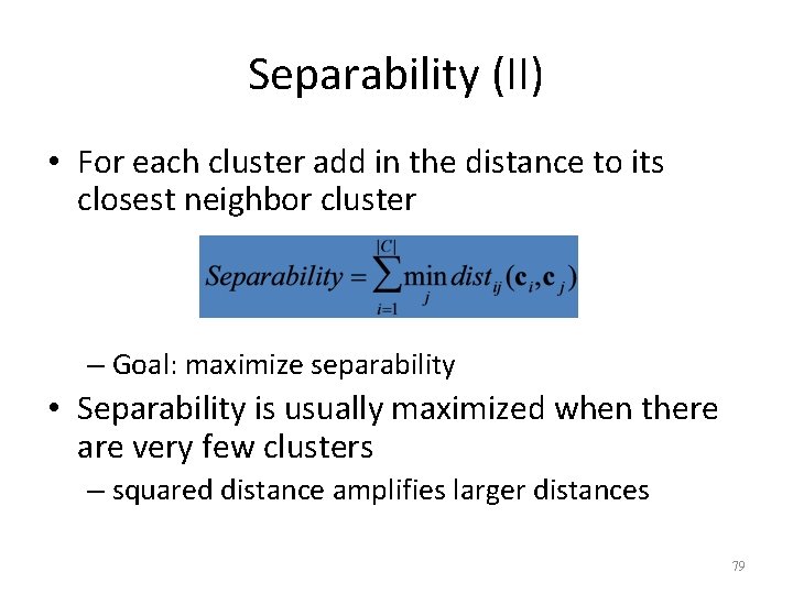
Separability (II) • For each cluster add in the distance to its closest neighbor cluster – Goal: maximize separability • Separability is usually maximized when there are very few clusters – squared distance amplifies larger distances 79

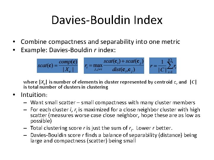
Davies-Bouldin Index • Combine compactness and separability into one metric • Example: Davies-Bouldin r index: where |Xc| is number of elements in cluster represented by centroid c, and |C| is total number of clusters in clustering • Intuition: – Want small scatter – small compactness with many cluster members – For each cluster i, ri is maximized for a close neighbor cluster with high scatter (measures worse case close neighbor, hope these are as low as possible) – Total clustering score r is just the sum of ri. Lower r better. – Davies-Bouldin score r finds a balance of separability (distance) being large and compactness (scatter) being small

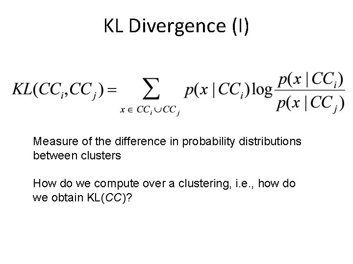
KL Divergence (I) Measure of the difference in probability distributions between clusters How do we compute over a clustering, i. e. , how do we obtain KL(CC)?

KL Divergence (II) • Compute KL as follows: (one possibility) 1. For each cluster a) Randomly split cluster in half b) Compute resulting KL 2. Repeat step 1 N times and compute average 3. Sum averages of all clusters to produce the KL of the clustering

Summary • Two types of evaluation – External – Internal • Various metrics have been proposed • Handle with care – Depends on the application – Some element of subjectivity

Final Comment on Cluster Validity “The validation of clustering structures is the most difficult and frustrating part of cluster analysis. Without a strong effort in this direction, cluster analysis will remain a black art accessible only to those true believers who have experience and great courage. ” Algorithms for Clustering Data, Jain and Dubes