Unsupervised Learning and Clustering In unsupervised learning you

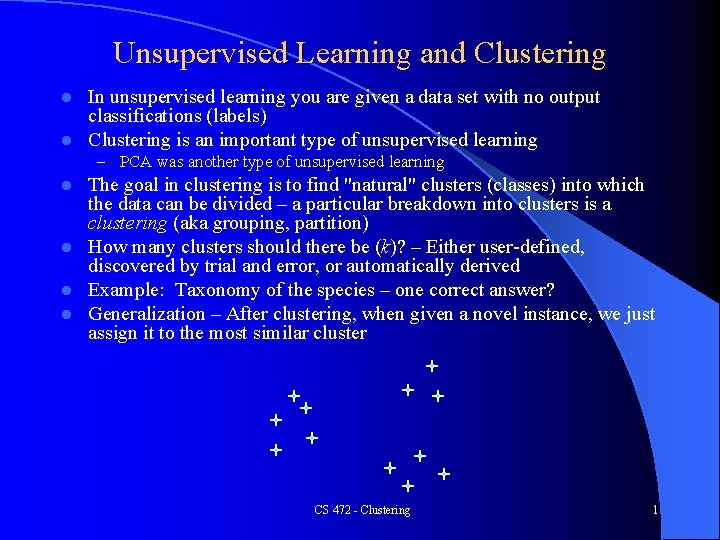
Unsupervised Learning and Clustering In unsupervised learning you are given a data set with no output classifications (labels) l Clustering is an important type of unsupervised learning l – PCA was another type of unsupervised learning The goal in clustering is to find "natural" clusters (classes) into which the data can be divided – a particular breakdown into clusters is a clustering (aka grouping, partition) l How many clusters should there be (k)? – Either user-defined, discovered by trial and error, or automatically derived l Example: Taxonomy of the species – one correct answer? l Generalization – After clustering, when given a novel instance, we just assign it to the most similar cluster l CS 472 - Clustering 1

Clustering How do we decide which instances should be in which cluster? l Typically put data which is "similar" into the same cluster l – Similarity is measured with some distance metric Also try to maximize between-class dissimilarity l Seek balance of within-class similarity and between-class dissimilarity l Similarity Metrics l – – Euclidean Distance most common for real valued instances Can use (1, 0) distance for nominal and unknowns like with k-NN Can create arbitrary distance metrics based on the task Important to normalize the input data CS 472 - Clustering 2

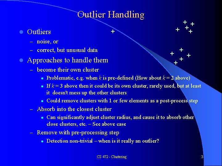
Outlier Handling l Outliers – noise, or – correct, but unusual data l Approaches to handle them – become their own cluster l Problematic, e. g. when k is pre-defined (How about k = 2 above) l If k = 3 above then it could be its own cluster, rarely used, but at least it doesn't mess up the other clusters l Could remove clusters with 1 or few elements as a post-process step – Absorb into the closest cluster l Can significantly adjust cluster radius, and cause it to absorb other close clusters, etc. – See above case – Remove with pre-processing step l Detection non-trivial – when is it really an outlier? CS 472 - Clustering 3

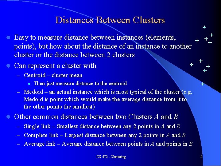
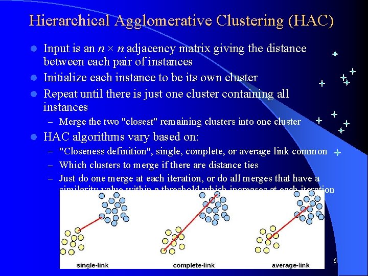
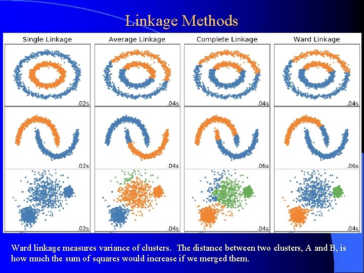
Distances Between Clusters Easy to measure distance between instances (elements, points), but how about the distance of an instance to another cluster or the distance between 2 clusters l Can represent a cluster with l – Centroid – cluster mean l Then just measure distance to the centroid – Medoid – an actual instance which is most typical of the cluster (e. g. Medoid is point which would make the average distance from it to the other points the smallest) l Other common distances between two Clusters A and B – Single link – Smallest distance between any 2 points in A and B – Complete link – Largest distance between any 2 points in A and B – Average link – Average distance between points in A and points in B CS 472 - Clustering 4

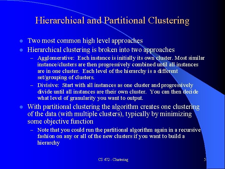
Hierarchical and Partitional Clustering Two most common high level approaches l Hierarchical clustering is broken into two approaches l – Agglomerative: Each instance is initially its own cluster. Most similar instance/clusters are then progressively combined until all instances are in one cluster. Each level of the hierarchy is a different set/grouping of clusters. – Divisive: Start with all instances as one cluster and progressively divide until all instances are their own cluster. You can then decide what level of granularity you want to output. l With partitional clustering the algorithm creates one clustering of the data (with multiple clusters), typically by minimizing some objective function – Note that you could run the partitional algorithm again in a recursive fashion on any or all of the new clusters if you want to build a hierarchy CS 472 - Clustering 5

Hierarchical Agglomerative Clustering (HAC) Input is an n × n adjacency matrix giving the distance between each pair of instances l Initialize each instance to be its own cluster l Repeat until there is just one cluster containing all instances l – Merge the two "closest" remaining clusters into one cluster l HAC algorithms vary based on: – "Closeness definition", single, complete, or average link common – Which clusters to merge if there are distance ties – Just do one merge at each iteration, or do all merges that have a similarity value within a threshold which increases at each iteration CS 472 - Clustering 6

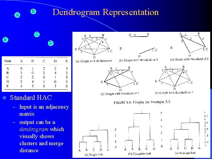
A Dendrogram Representation B C E l D Standard HAC – Input is an adjacency matrix – output can be a dendrogram which visually shows clusters and merge distance CS 472 - Clustering 7

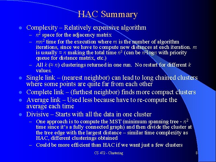
HAC Summary l Complexity – Relatively expensive algorithm – n 2 space for the adjacency matrix – mn 2 time for the execution where m is the number of algorithm iterations, since we have to compute new distances at each iteration. m is usually ≈ n making the total time n 3 (can be n 2 logn with priority queue for distance matrix, etc. ) – All k (≈ n) clusterings returned in one run. No restart for different k values. Single link – (nearest neighbor) can lead to long chained clusters where some points are quite far from each other l Complete link – (farthest neighbor) finds more compact clusters l Average link – Used less because have to re-compute the average each time l Divisive – Starts with all the data in one cluster l – One approach is to compute the MST (minimum spanning tree - n 2 time since it’s a fully connected graph) and then divide the cluster at the tree edge with the largest distance – similar time complexity as HAC, different clusterings obtained – Could be more efficient than HAC if we want just a few clusters CS 472 - Clustering 8

Linkage Methods Ward linkage measures variance of clusters. The distance between two clusters, A and B, is how much the sum of squares would increase if we merged them.

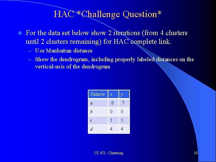
HAC *Challenge Question* l For the data set below show 2 iterations (from 4 clusters until 2 clusters remaining) for HAC complete link. – Use Manhattan distance – Show the dendrogram, including properly labeled distances on the vertical-axis of the dendrogram Pattern x y a . 8 . 7 b 0 0 c 1 1 d 4 4 CS 472 - Clustering 10

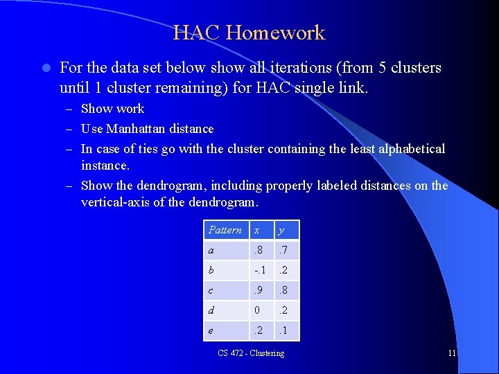
HAC Homework l For the data set below show all iterations (from 5 clusters until 1 cluster remaining) for HAC single link. – Show work – Use Manhattan distance – In case of ties go with the cluster containing the least alphabetical instance. – Show the dendrogram, including properly labeled distances on the vertical-axis of the dendrogram. Pattern x y a . 8 . 7 b -. 1 . 2 c . 9 . 8 d 0 . 2 e . 2 . 1 CS 472 - Clustering 11

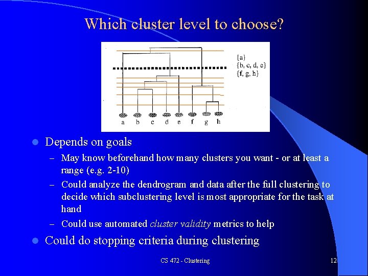
Which cluster level to choose? l Depends on goals – May know beforehand how many clusters you want - or at least a range (e. g. 2 -10) – Could analyze the dendrogram and data after the full clustering to decide which subclustering level is most appropriate for the task at hand – Could use automated cluster validity metrics to help l Could do stopping criteria during clustering CS 472 - Clustering 12

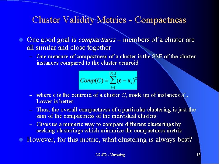
Cluster Validity Metrics - Compactness l One good goal is compactness – members of a cluster are all similar and close together – One measure of compactness of a cluster is the SSE of the cluster instances compared to the cluster centroid – where c is the centroid of a cluster C, made up of instances Xc. Lower is better. – Thus, the overall compactness of a particular clustering is just the sum of the compactness of the individual clusters – Gives us a numeric way to compare different clusterings by seeking clusterings which minimize the compactness metric l However, for this metric, what clustering is always best? CS 472 - Clustering 13

Cluster Validity Metrics - Separability l Another good goal is separability – members of one cluster are sufficiently different from members of another cluster (cluster dissimilarity) – One measure of the separability of two clusters is their squared distance. The bigger the distance the better. – distij = (ci - cj)2 where ci and cj are two cluster centroids – For a clustering which cluster distances should we compare? CS 472 - Clustering 14

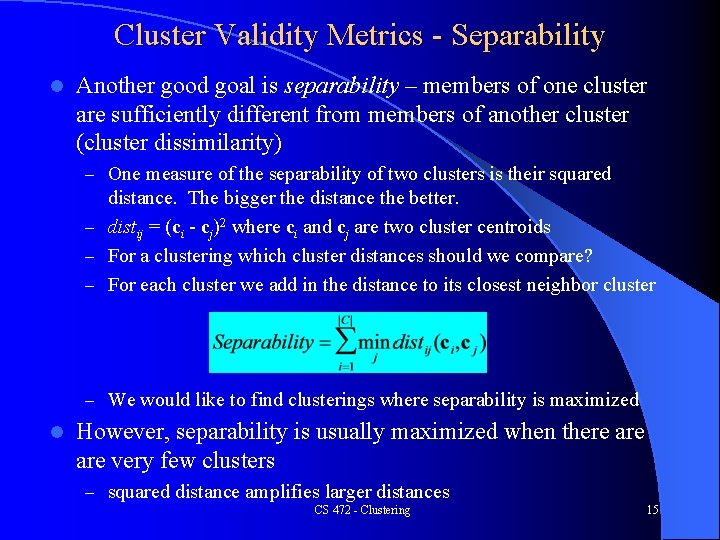
Cluster Validity Metrics - Separability l Another good goal is separability – members of one cluster are sufficiently different from members of another cluster (cluster dissimilarity) – One measure of the separability of two clusters is their squared distance. The bigger the distance the better. – distij = (ci - cj)2 where ci and cj are two cluster centroids – For a clustering which cluster distances should we compare? – For each cluster we add in the distance to its closest neighbor cluster – We would like to find clusterings where separability is maximized l However, separability is usually maximized when there are very few clusters – squared distance amplifies larger distances CS 472 - Clustering 15

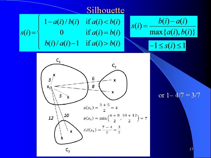
Silhouette Want techniques that find a balance between inter-cluster similarity and intra-cluster dissimilarity l Silhouette is one good popular approach l Start with a clustering, using any clustering algorithm, which has k unique clusters l a(i) = average dissimilarity of instance i to all other instances in the cluster to which i is assigned – Want it small l – Dissimilarity could be Euclidian distance, etc. b(i) = the smallest (comparing each different cluster) average dissimilarity of instance i to all instances in that cluster – Want it large l b(i) is smallest for the best different cluster that i could be assigned to – the best cluster that you would move i to if needed l CS 472 - Clustering 16

Silhouette or 1– 4/7 = 3/7 CS 472 - Clustering 17

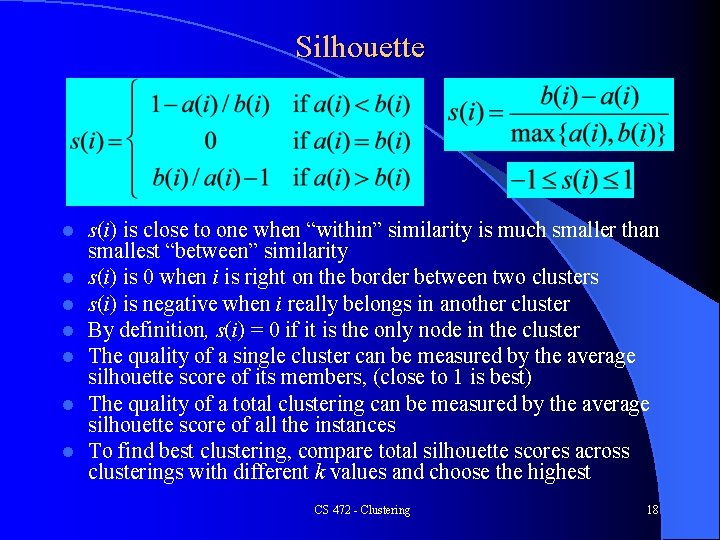
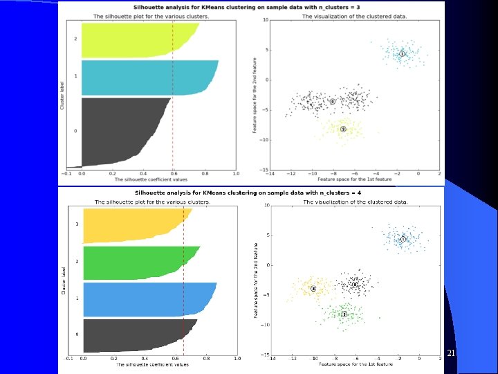
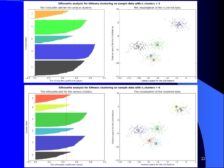
Silhouette l l l l s(i) is close to one when “within” similarity is much smaller than smallest “between” similarity s(i) is 0 when i is right on the border between two clusters s(i) is negative when i really belongs in another cluster By definition, s(i) = 0 if it is the only node in the cluster The quality of a single cluster can be measured by the average silhouette score of its members, (close to 1 is best) The quality of a total clustering can be measured by the average silhouette score of all the instances To find best clustering, compare total silhouette scores across clusterings with different k values and choose the highest CS 472 - Clustering 18

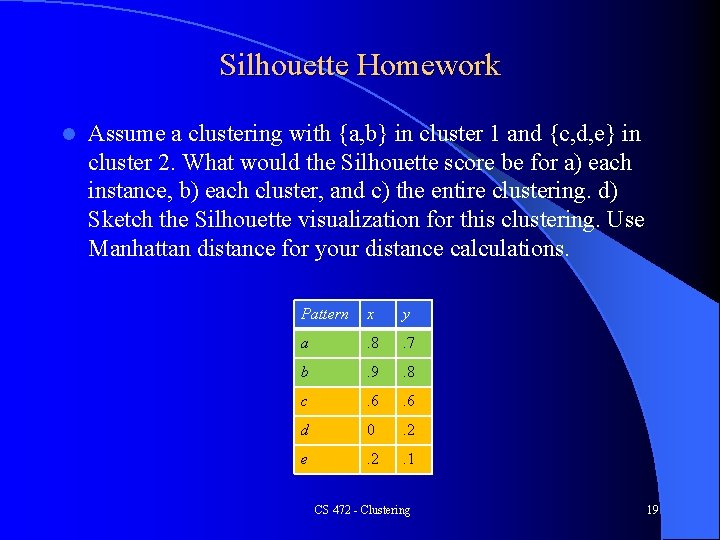
Silhouette Homework l Assume a clustering with {a, b} in cluster 1 and {c, d, e} in cluster 2. What would the Silhouette score be for a) each instance, b) each cluster, and c) the entire clustering. d) Sketch the Silhouette visualization for this clustering. Use Manhattan distance for your distance calculations. Pattern x y a . 8 . 7 b . 9 . 8 c . 6 d 0 . 2 e . 2 . 1 CS 472 - Clustering 19

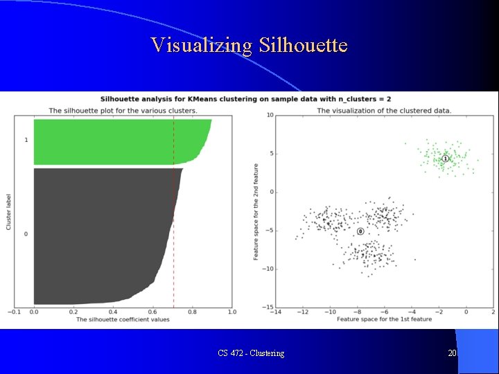
Visualizing Silhouette CS 472 - Clustering 20

CS 472 - Clustering 21

CS 472 - Clustering 22

Silhouette l Best case graph for silhouette? CS 472 - Clustering 23

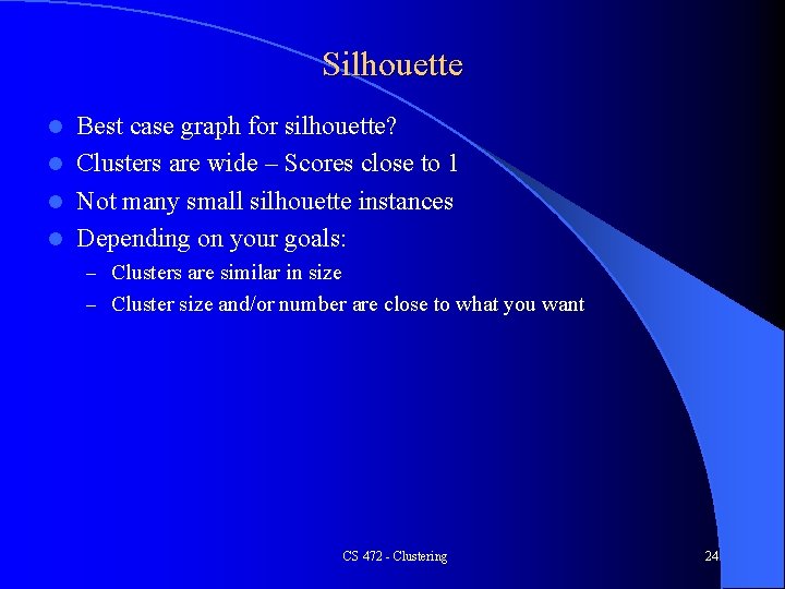
Silhouette Best case graph for silhouette? l Clusters are wide – Scores close to 1 l Not many small silhouette instances l Depending on your goals: l – Clusters are similar in size – Cluster size and/or number are close to what you want CS 472 - Clustering 24

Silhouette l Can just use total silhouette average to decide best clustering but best to do silhouette analysis with a visualization tool and use score along with other aspects of the clustering – – Cluster sizes Number of clusters Shape of clusters Etc. Note when task dimensions are > 3 (typical and no longer visualizable for us), silhouette graph still easy to visualize l O(n 2) complexity due to b(i) computation l There are other cluster metrics out there l These metrics are rough guidelines and should be "taken with a grain of salt" l CS 472 - Clustering 25

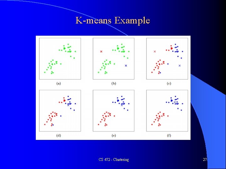
k-means l Perhaps the most well known clustering algorithm – Partitioning algorithm – Must choose a k beforehand – Thus, typically try a spread of different k's (e. g. 2 -10) and then compare results to see which made the best clustering l Could use cluster validity metrics (e. g. Silhouette) to help in the decision Randomly choose k instances from the data set to be the initial k centroids 2. Repeat until no (or negligible) more changes occur 1. a) Group each instance with its closest centroid b) Recalculate the centroid based on its new cluster l Time complexity is O(mkn) where m is # of iterations and space is O(n), both much better than HAC time and space (n 3 and n 2) CS 472 - Clustering 26

K-means Example CS 472 - Clustering 27

k-means Continued l Type of EM (Expectation-Maximization) algorithm, Gradient descent – Can struggle with local minima, unlucky random initial centroids, and outliers l K-medoids finds medoid (median) centers rather than average centers and is thus less effected by outliers – Local minima, empty clusters: Can just re-run with different initial centroids l l l Could compare different solutions for a specific k value by seeing which clusterings minimize the overall SSE to the cluster centers (i. e. compactness) or use silhouette, etc. And test solutions with different k values using Silhouette or other metric Can do further refinement of HAC results using any k centroids from HAC as starting centroids for k-means CS 472 - Clustering 28

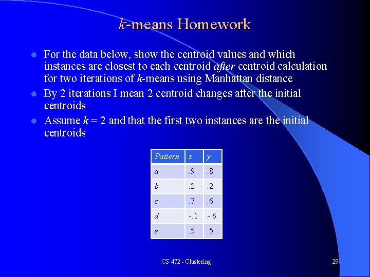
k-means Homework For the data below, show the centroid values and which instances are closest to each centroid after centroid calculation for two iterations of k-means using Manhattan distance l By 2 iterations I mean 2 centroid changes after the initial centroids l Assume k = 2 and that the first two instances are the initial centroids l Pattern x y a . 9 . 8 b . 2 c . 7 . 6 d -. 1 -. 6 e . 5 CS 472 - Clustering 29

Clustering Project l Last individual project CS 472 - Clustering 30

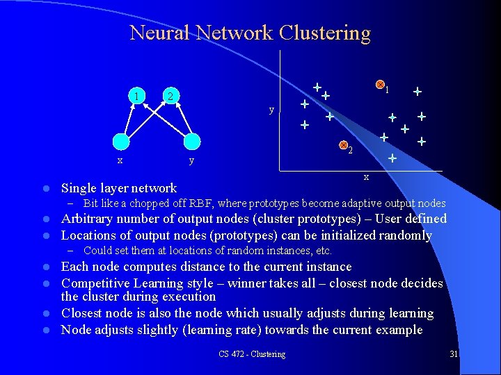
Neural Network Clustering 1 × 1 2 y x l × 2 y x Single layer network – Bit like a chopped off RBF, where prototypes become adaptive output nodes l l Arbitrary number of output nodes (cluster prototypes) – User defined Locations of output nodes (prototypes) can be initialized randomly – Could set them at locations of random instances, etc. Each node computes distance to the current instance Competitive Learning style – winner takes all – closest node decides the cluster during execution l Closest node is also the node which usually adjusts during learning l Node adjusts slightly (learning rate) towards the current example l l CS 472 - Clustering 31

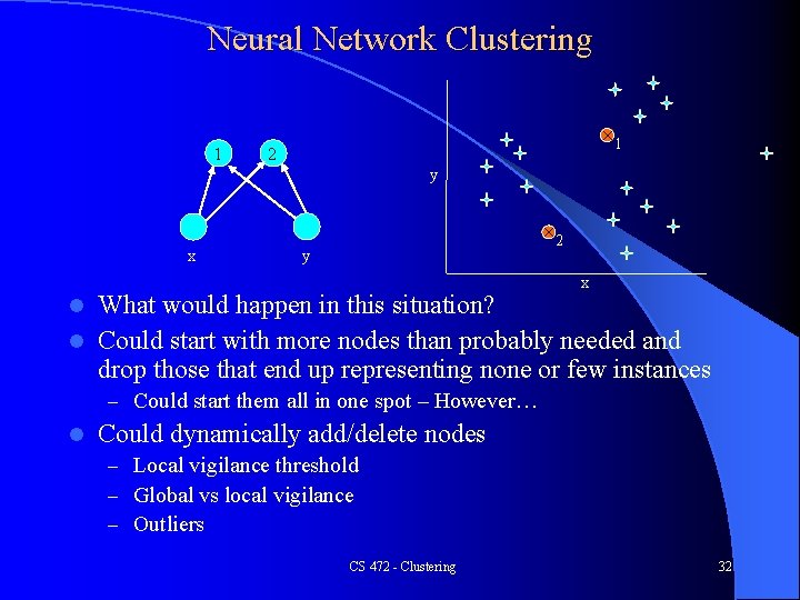
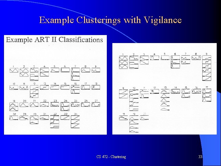
Neural Network Clustering 1 × 1 2 y x × 2 y x What would happen in this situation? l Could start with more nodes than probably needed and drop those that end up representing none or few instances l – Could start them all in one spot – However… l Could dynamically add/delete nodes – Local vigilance threshold – Global vs local vigilance – Outliers CS 472 - Clustering 32

Example Clusterings with Vigilance CS 472 - Clustering 33

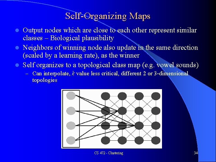
Self-Organizing Maps Output nodes which are close to each other represent similar classes – Biological plausibility l Neighbors of winning node also update in the same direction (scaled by a learning rate), as the winner l Self organizes to a topological class map (e. g. vowel sounds) l – Can interpolate, k value less critical, different 2 or 3 -dimensional topologies CS 472 - Clustering 34

Other Unsupervised Models Vector Quantization – Discretize into codebooks l K-medoids l Conceptual Clustering (Symbolic AI) – Cobweb, Classit, etc. l – Incremental vs Batch Density mixtures l Interactive clustering l Special models for large data bases – n 2 space? , disk I/O l – Sampling – Bring in enough data to fill memory and then cluster – Once initial prototypes found, can iteratively bring in more data to adjust/fine-tune the prototypes as desired – Linear algorithms CS 472 - Clustering 35

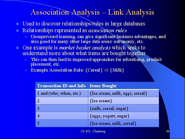
Association Analysis – Link Analysis l l Used to discover relationships/rules in large databases Relationships represented as association rules – Unsupervised learning, can give significant business advantages, and also good for many other large data areas: astronomy, etc. l One example is market basket analysis which seeks to understand more about what items are bought together – This can then lead to improved approaches for advertising, product placement, etc. – Example Association Rule: {Cereal} {Milk} Transaction ID and Info Items Bought 1 and (who, when, etc. ) {Ice cream, milk, eggs, cereal} 2 {Ice cream} 3 {milk, cereal, sugar} 4 {eggs, yogurt, sugar} 5 {Ice cream, milk, cereal} CS 472 - Clustering 36

Summary l Can use clustering as a discretization technique on continuous data for many other models which favor nominal or discretized data – Including supervised learning models (Decision trees, Naïve Bayes, etc. ) l With so much (unlabeled) data out there, opportunities to do unsupervised learning are growing – Semi-Supervised learning is becoming very important – Use unlabeled data to augment the more limited labeled data to improve accuracy of a supervised learner l Deep Learning – Unsupervised training of early layers is an important approach in some deep learning models CS 472 - Clustering 37

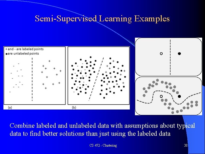
Semi-Supervised Learning Examples Combine labeled and unlabeled data with assumptions about typical data to find better solutions than just using the labeled data CS 472 - Clustering 38