Unsupervised Learning Neural Networks 11 Unsupervised learning simple

Unsupervised Learning Neural Networks 11

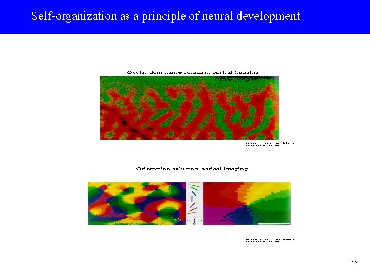
Unsupervised learning: simple competitive learning Biological background: Neurons are wired topographically, nearby neurons connect to nearby neurons. In visual cortex, neurons are organized in functional columns. How do these neurons organise? Don’t get any ‘supervision’ Ocular dominance columns: one region responds to one eye input Orientation columns: one region responds to one direction

Self-organization as a principle of neural development

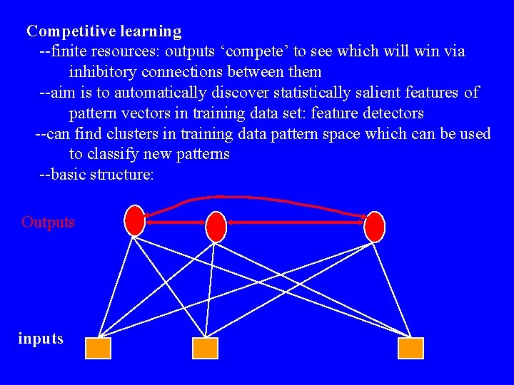
Competitive learning --finite resources: outputs ‘compete’ to see which will win via inhibitory connections between them --aim is to automatically discover statistically salient features of pattern vectors in training data set: feature detectors --can find clusters in training data pattern space which can be used to classify new patterns --basic structure: Outputs inputs

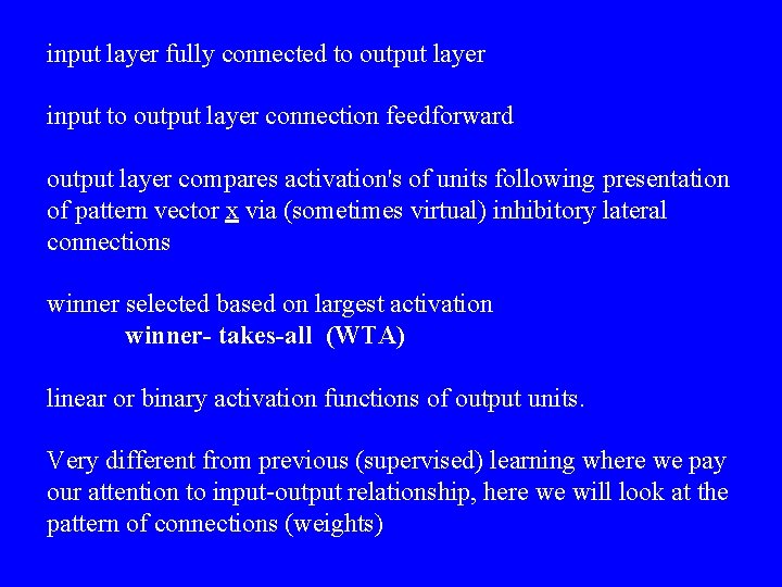
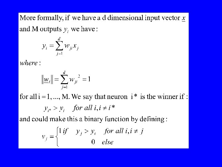
input layer fully connected to output layer input to output layer connection feedforward output layer compares activation's of units following presentation of pattern vector x via (sometimes virtual) inhibitory lateral connections winner selected based on largest activation winner- takes-all (WTA) linear or binary activation functions of output units. Very different from previous (supervised) learning where we pay our attention to input-output relationship, here we will look at the pattern of connections (weights)

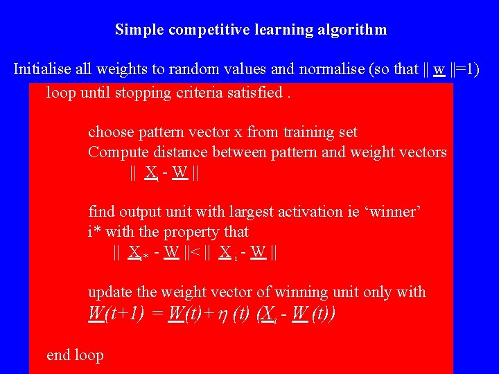
Simple competitive learning algorithm Initialise all weights to random values and normalise (so that || w ||=1) loop until stopping criteria satisfied. choose pattern vector x from training set Compute distance between pattern and weight vectors || Xi - W || find output unit with largest activation ie ‘winner’ i* with the property that || Xi* - W ||< || X i - W || update the weight vector of winning unit only with W(t+1) = W(t)+h (t) (Xi - W (t)) end loop

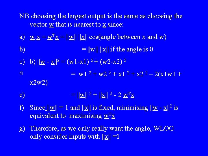
NB choosing the largest output is the same as choosing the vector w that is nearest to x since: a) w. x = w. Tx = ||w|| ||x|| cos(angle between x and w) b) = ||w|| ||x|| if the angle is 0 c) b) ||w - x||2 = (w 1 -x 1) 2 + (w 2 -x 2) 2 d) = w 1 2 + w 2 2 + x 1 2 + x 2 2 – 2(x 1 w 1 + x 2 w 2) e) = ||w|| 2 + ||x|| 2 - 2 w. Tx f) Since ||w|| = 1 and ||x|| is fixed, minimising ||w - x||2 is equivalent to maximising w. Tx g) Therefore, as we only really want the angle, WLOG only consider inputs with ||x|| =1

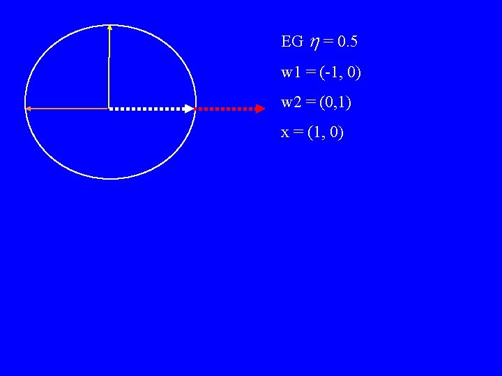
EG h = 0. 5 w 1 = (-1, 0) w 2 = (0, 1) x = (1, 0)

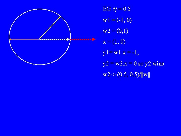
EG h = 0. 5 w 1 = (-1, 0) w 2 = (0, 1) x = (1, 0) y 1= w 1. x = -1, y 2 = w 2. x = 0 so y 2 wins w 2 -> (0. 5, 0. 5)/||w||

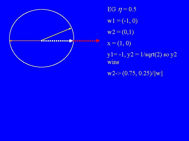
EG h = 0. 5 w 1 = (-1, 0) w 2 = (0, 1) x = (1, 0) y 1= -1, y 2 = 1/sqrt(2) so y 2 wins w 2 -> (0. 75, 0. 25)/||w||

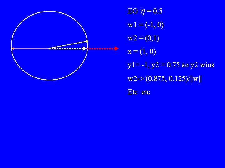
EG h = 0. 5 w 1 = (-1, 0) w 2 = (0, 1) x = (1, 0) y 1= -1, y 2 = 0. 75 so y 2 wins w 2 -> (0. 875, 0. 125)/||w|| Etc etc

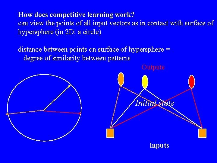
How does competitive learning work? can view the points of all input vectors as in contact with surface of hypersphere (in 2 D: a circle) distance between points on surface of hypersphere = degree of similarity between patterns Outputs Initial state inputs

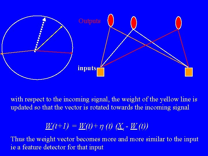
Outputs inputs with respect to the incoming signal, the weight of the yellow line is updated so that the vector is rotated towards the incoming signal W(t+1) = W(t)+h (t) (Xi - W (t)) Thus the weight vector becomes more and more similar to the input ie a feature detector for that input

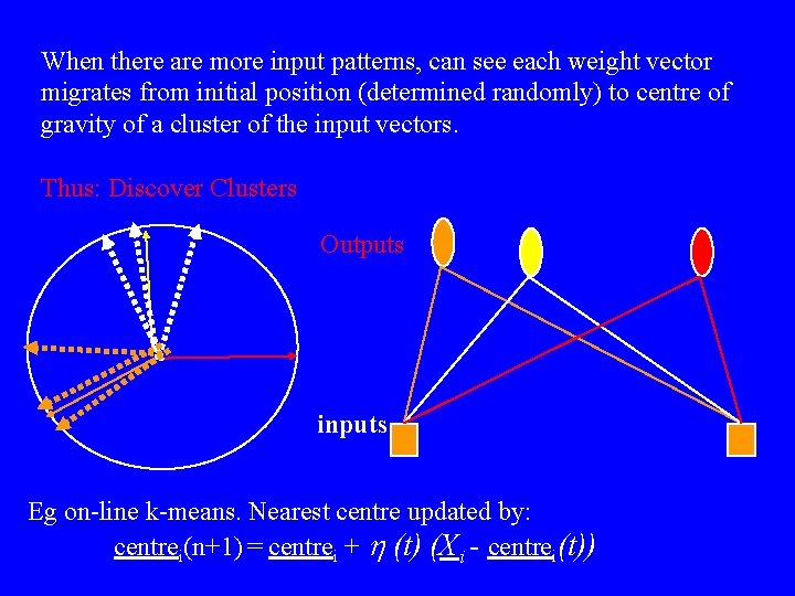
When there are more input patterns, can see each weight vector migrates from initial position (determined randomly) to centre of gravity of a cluster of the input vectors. Thus: Discover Clusters Outputs inputs Eg on-line k-means. Nearest centre updated by: centrei(n+1) = centrei + h (t) (Xi - centrei(t))

Matlab demo

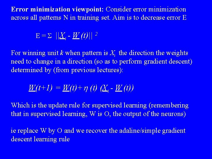
Error minimization viewpoint: Consider error minimization across all patterns N in training set. Aim is to decrease error E E = S ||Xi - W (t)|| 2 For winning unit k when pattern is Xi the direction the weights need to change in a direction (so as to perform gradient descent) determined by (from previous lectures): W(t+1) = W(t)+h (t) (Xi - W (t)) Which is the update rule for supervised learning (remembering that in supervised learning, W is O, the output of the neurons) ie replace W by O and we recover the adaline/simple gradient descent learning rule

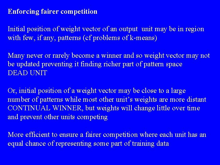
Enforcing fairer competition Initial position of weight vector of an output unit may be in region with few, if any, patterns (cf problems of k-means) Many never or rarely become a winner and so weight vector may not be updated preventing it finding richer part of pattern space DEAD UNIT Or, initial position of a weight vector may be close to a large number of patterns while most other unit’s weights are more distant CONTINUAL WINNER, but weights will change little over time and prevent other units competing More efficient to ensure a fairer competition where each unit has an equal chance of representing some part of training data

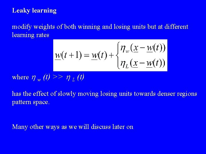
Leaky learning modify weights of both winning and losing units but at different learning rates where h w (t) >> h L (t) has the effect of slowly moving losing units towards denser regions pattern space. Many other ways as we will discuss later on

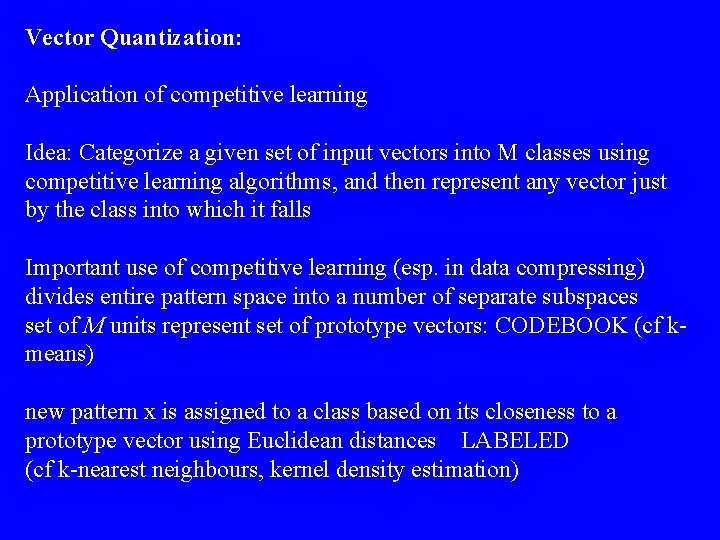
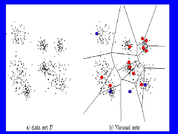
Vector Quantization: Application of competitive learning Idea: Categorize a given set of input vectors into M classes using competitive learning algorithms, and then represent any vector just by the class into which it falls Important use of competitive learning (esp. in data compressing) divides entire pattern space into a number of separate subspaces set of M units represent set of prototype vectors: CODEBOOK (cf kmeans) new pattern x is assigned to a class based on its closeness to a prototype vector using Euclidean distances LABELED (cf k-nearest neighbours, kernel density estimation)

Example (VQ) See: http: //www. neuroinformatik. ruhr-uni-bochum. de/ini/VDM/research/gsn/Demo. GNG/GNG. html

Topographic maps Extend the ideas of competitive learning to incorporate the neighborhood around inputs and neurons We want a nonlinear transformation of input pattern space onto output feature space which preserves neighbourhood relationship between the inputs -- a feature map where nearby neurons respond to similar inputs Eg Place cells, orientation columns, somatosensory cells etc Idea is that neurons selectively tune to particular input patterns in such a way that the neurons become ordered with respect to each other so that a meaningful coordinate system for different input features is created

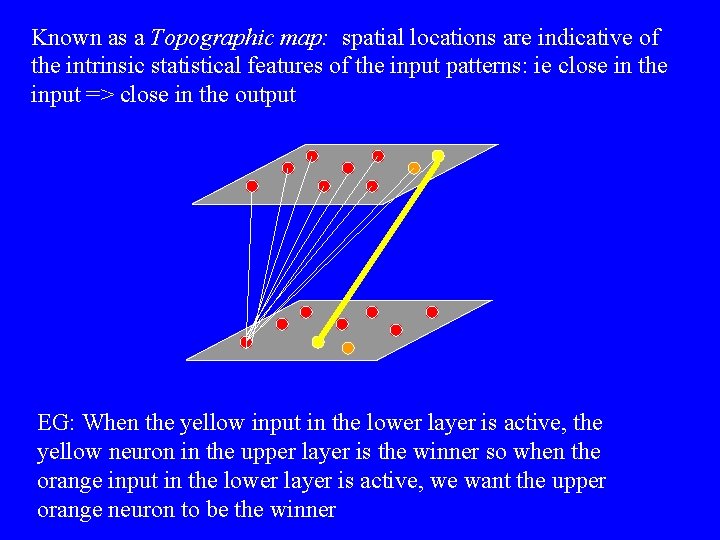
Known as a Topographic map: spatial locations are indicative of the intrinsic statistical features of the input patterns: ie close in the input => close in the output EG: When the yellow input in the lower layer is active, the yellow neuron in the upper layer is the winner so when the orange input in the lower layer is active, we want the upper orange neuron to be the winner

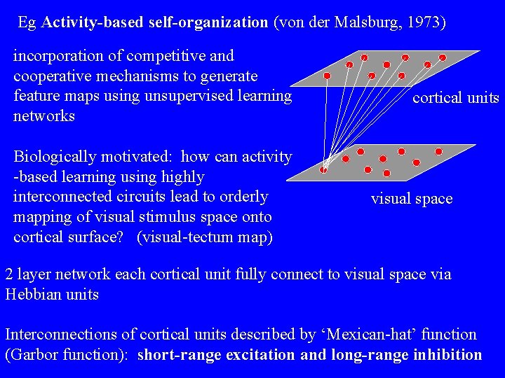
Eg Activity-based self-organization (von der Malsburg, 1973) incorporation of competitive and cooperative mechanisms to generate feature maps using unsupervised learning networks Biologically motivated: how can activity -based learning using highly interconnected circuits lead to orderly mapping of visual stimulus space onto cortical surface? (visual-tectum map) cortical units visual space 2 layer network each cortical unit fully connect to visual space via Hebbian units Interconnections of cortical units described by ‘Mexican-hat’ function (Garbor function): short-range excitation and long-range inhibition

After learning (see original paper for details), a topographic map appears. However, input dimension is the same as output dimension Kohonen simplified this model and called it Kohonen’s self-organizing map (SOM) algorithm More general as it can perform dimensionality reduction SOM can be viewed as a vector quantisation type algorithm

The idea in an SOM is to transform on input of arbitrary dimension into a 1 or 2 dimensional discrete map Again, 2 layers of neurons with all inputs connecting to each output Output neurons are held in a one or (usually) 2 D lattice, where position in the lattice defines the distance between the neurons Once weights of net initialised, algorithm comprises 3 processes: 1. Competition. Given an input pattern, outputs compete to see who is winner based on a discriminant function (eg similarity of input vector and weight vector) 2. Cooperation. Winning neuron determines spatial location of a topological neighborhood within which output neurons excited 3. Synaptic Adaptation. Excite neurons adapt weights so that value of discrimant function increases ie so that presenting a similar input would result in enhanced response from winner

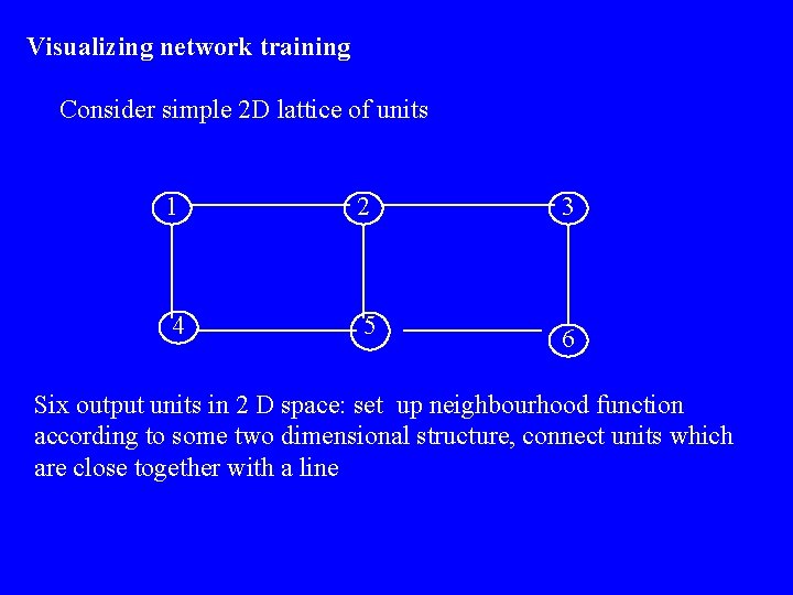
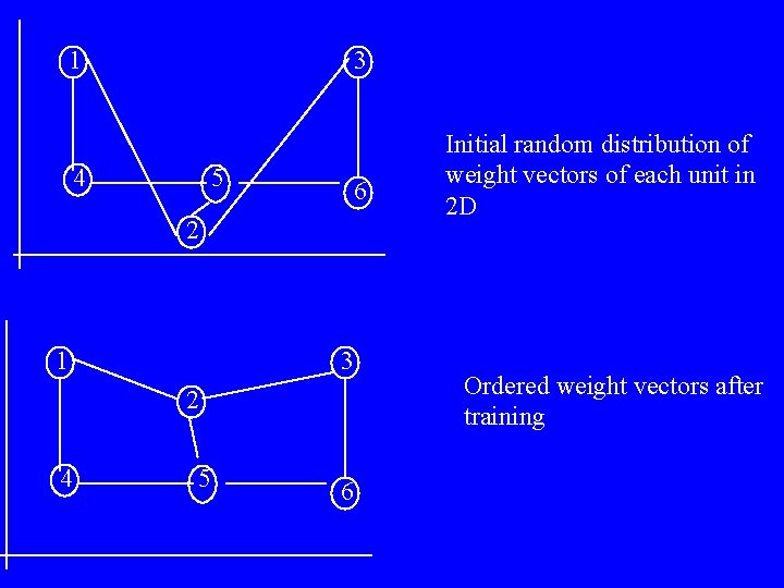
Visualizing network training Consider simple 2 D lattice of units 1 2 3 4 5 6 Six output units in 2 D space: set up neighbourhood function according to some two dimensional structure, connect units which are close together with a line

1 3 4 5 6 2 1 3 2 4 5 6 Initial random distribution of weight vectors of each unit in 2 D Ordered weight vectors after training

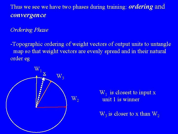
Thus we see we have two phases during training: ordering and convergence Ordering Phase -Topographic ordering of weight vectors of output units to untangle map so that weight vectors are evenly spread and in their natural order eg W 1 x W 3 W 2 W 1 is closest to input x unit 1 is winner W 3 is closer to x than W 2

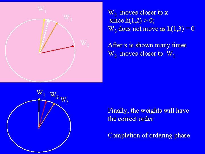
W 1 W 2 moves closer to x since h(1, 2) > 0; W 3 does not move as h(1, 3) = 0 W 3 W 2 W 1 W 2 After x is shown many times W 2 moves closer to W 1 W 3 Finally, the weights will have the correct order Completion of ordering phase

Convergence phase Topographic map adapts to probability density of input patterns in training data However, it is important that ordering is maintained Thus learning rate should be small to prevent large movements of weight vector but non-zero to avoid pathological states (getting caught in odd minima etc) Neighbourhood size should also start off relatively small containing only close neighbours and eventually shrinking to nearest neighbours (or less)

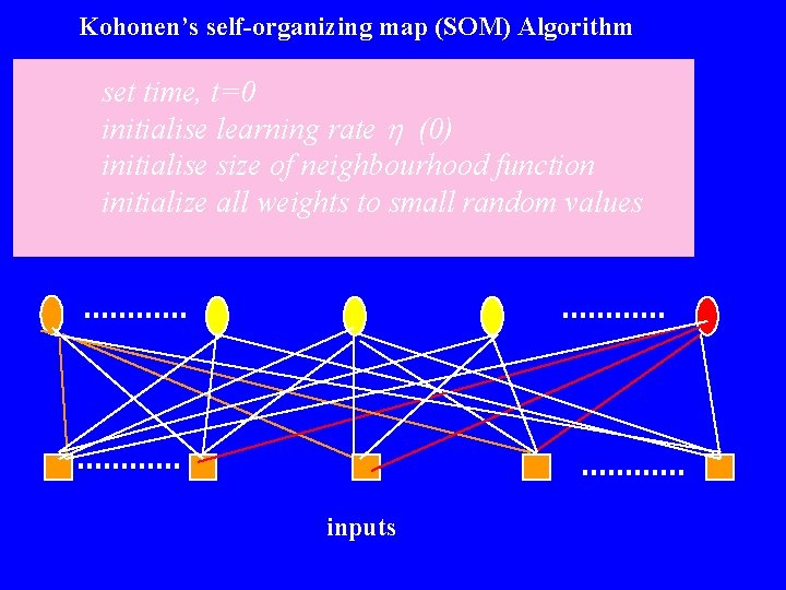
Kohonen’s self-organizing map (SOM) Algorithm set time, t=0 initialise learning rate h (0) initialise size of neighbourhood function initialize all weights to small random values inputs

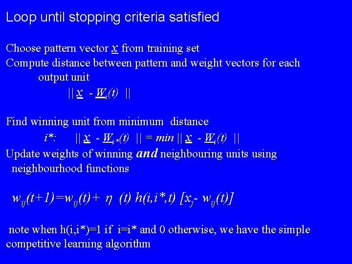
Loop until stopping criteria satisfied Choose pattern vector x from training set Compute distance between pattern and weight vectors for each output unit || x - Wi(t) || Find winning unit from minimum distance i*: || x - Wi*(t) || = min || x - Wi(t) || Update weights of winning and neighbouring units using neighbourhood functions wij(t+1)=wij(t)+ h (t) h(i, i*, t) [xj- wij(t)] note when h(i, i*)=1 if i=i* and 0 otherwise, we have the simple competitive learning algorithm

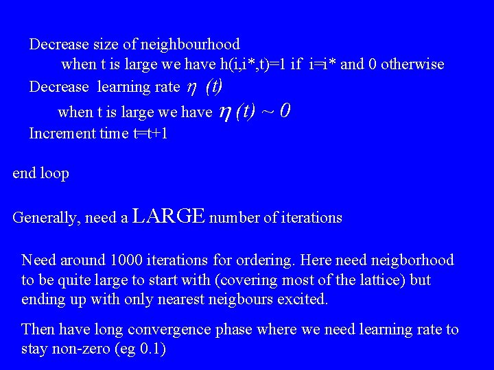
Decrease size of neighbourhood when t is large we have h(i, i*, t)=1 if i=i* and 0 otherwise Decrease learning rate h (t) when t is large we have h Increment time t=t+1 (t) ~ 0 end loop Generally, need a LARGE number of iterations Need around 1000 iterations for ordering. Here need neigborhood to be quite large to start with (covering most of the lattice) but ending up with only nearest neigbours excited. Then have long convergence phase where we need learning rate to stay non-zero (eg 0. 1)

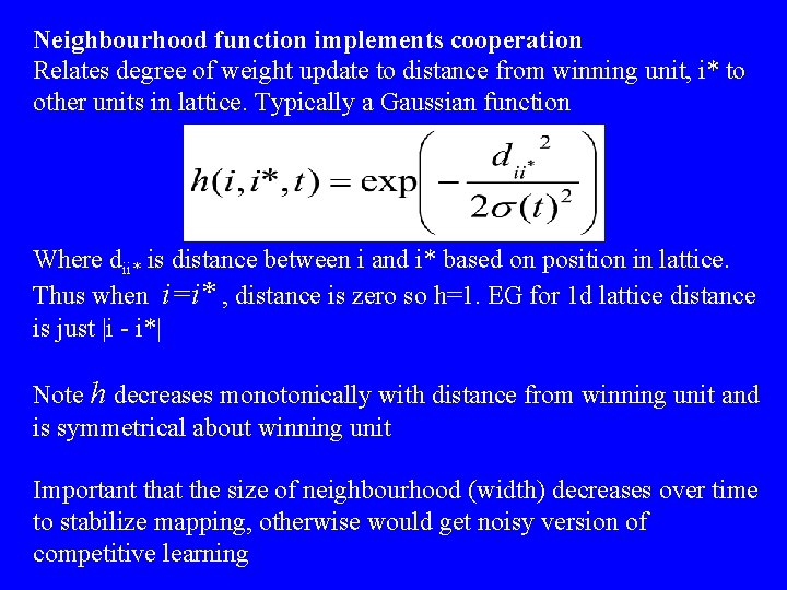
Neighbourhood function implements cooperation Relates degree of weight update to distance from winning unit, i* to other units in lattice. Typically a Gaussian function Where dii* is distance between i and i* based on position in lattice. Thus when i=i* , distance is zero so h=1. EG for 1 d lattice distance is just |i - i*| Note h decreases monotonically with distance from winning unit and is symmetrical about winning unit Important that the size of neighbourhood (width) decreases over time to stabilize mapping, otherwise would get noisy version of competitive learning

Biologically, development (self-organization) is governed by the gradient of a chemical element, which generally preserves the topological relation. Kohonen (and others) has shown that the neighborhood function could be implemented by a difusing neuromodulatory gas such as nitric oxide (which has been shown to be necessary for learning esp. spatial learning) Thus there is some biological motivation for the SOM

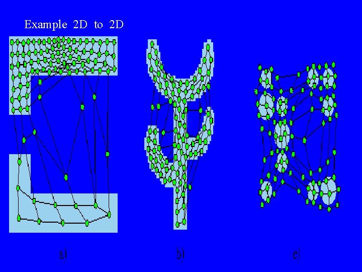
Example 2 D to 2 D

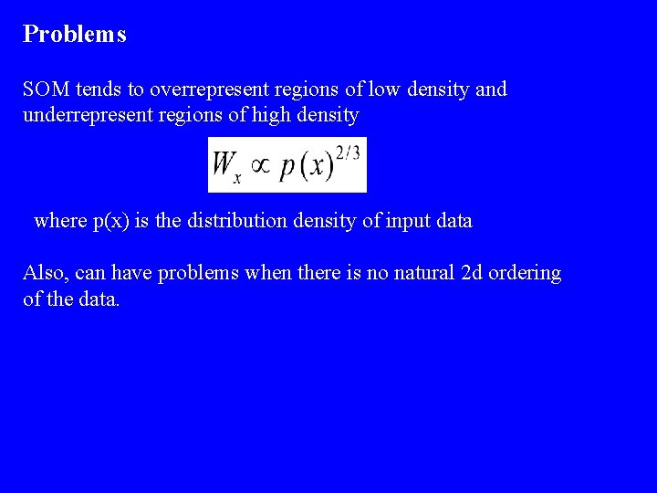
Problems SOM tends to overrepresent regions of low density and underrepresent regions of high density where p(x) is the distribution density of input data Also, can have problems when there is no natural 2 d ordering of the data.

Example (JAVA) See: http: //www. neuroinformatik. ruhr-unibochum. de/ini/VDM/research/gsn/Demo. GNG/GNG. html