THE NCEP CLIMATE FORECAST SYSTEM REANALYSIS THE ENVIRONMENTAL

THE NCEP CLIMATE FORECAST SYSTEM REANALYSIS THE ENVIRONMENTAL MODELING CENTER NCEP/NWS/NOAA

The NCEP Climate Forecast System Reanalysis Suranjana Saha, Shrinivas Moorthi, Hua-Lu Pan, Xingren Wu, Jiande Wang, Sudhir Nadiga, Patrick Tripp, Robert Kistler, John Woollen, David Behringer, Haixia Liu, Diane Stokes, Robert Grumbine, George Gayno, Jun Wang, Yu-Tai Hou, Hui-ya Chuang, Hann. Ming H. Juang, Joe Sela, Mark Iredell, Russ Treadon, Daryl Kleist, Paul Van Delst, Dennis Keyser, John Derber, Michael Ek, Jesse Meng, Helin Wei, Rongqian Yang, Stephen Lord, Huug van den Dool, Arun Kumar, Wanqiu Wang, Craig Long, Muthuvel Chelliah, Yan Xue, Boyin Huang, Jae-Kyung Schemm, Wesley Ebisuzaki, Roger Lin, Pingping Xie, Mingyue Chen, Shuntai Zhou, Wayne Higgins, Cheng-Zhi Zou, Quanhua Liu, Yong Chen, Yong Han, Lidia Cucurull, Richard W. Reynolds, Glenn Rutledge, Mitch Goldberg Bulletin of the American Meteorological Society Volume 91, Issue 8, pp 1015 -1057. doi: 10. 1175/2010 BAMS 3001. 1

• WHAT IS AN ANALYSIS SYSTEM? • WHAT IS A REANALYSIS SYSTEM ?

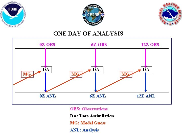
ONE DAY OF ANALYSIS 0 Z OBS MG DA 0 Z ANL 6 Z OBS MG DA 6 Z ANL OBS: Observations DA: Data Assimilation MG: Model Guess ANL: Analysis 12 Z OBS MG DA 12 Z ANL

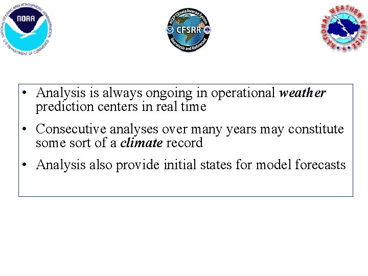
• Analysis is always ongoing in operational weather prediction centers in real time • Consecutive analyses over many years may constitute some sort of a climate record • Analysis also provide initial states for model forecasts

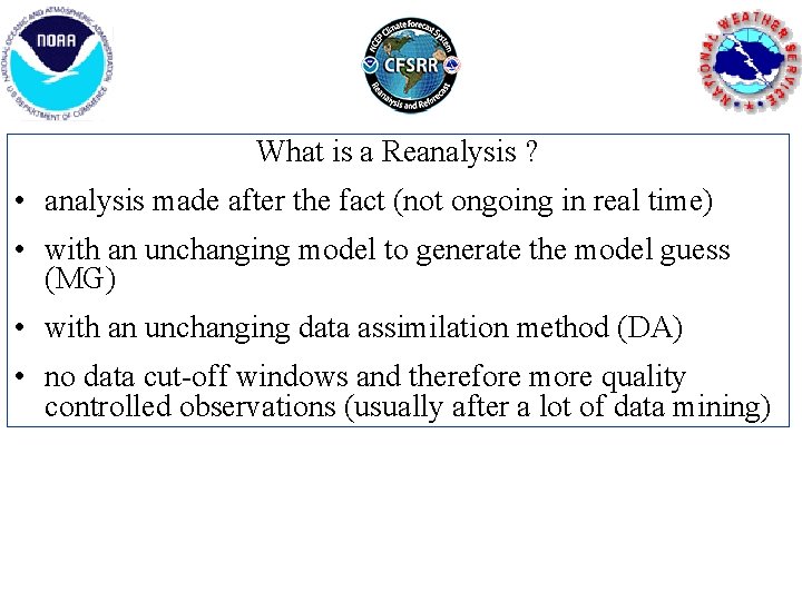
What is a Reanalysis ? • analysis made after the fact (not ongoing in real time) • with an unchanging model to generate the model guess (MG) • with an unchanging data assimilation method (DA) • no data cut-off windows and therefore more quality controlled observations (usually after a lot of data mining)

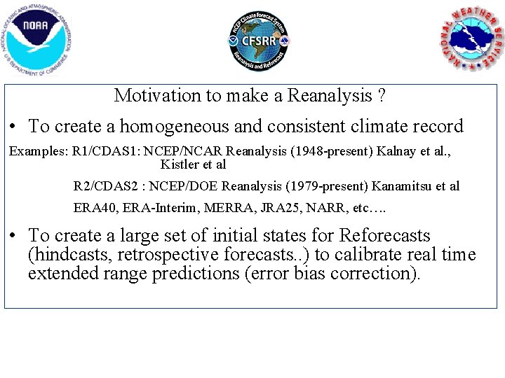
Motivation to make a Reanalysis ? • To create a homogeneous and consistent climate record Examples: R 1/CDAS 1: NCEP/NCAR Reanalysis (1948 -present) Kalnay et al. , Kistler et al R 2/CDAS 2 : NCEP/DOE Reanalysis (1979 -present) Kanamitsu et al ERA 40, ERA-Interim, MERRA, JRA 25, NARR, etc…. • To create a large set of initial states for Reforecasts (hindcasts, retrospective forecasts. . ) to calibrate real time extended range predictions (error bias correction).

An upgrade to the NCEP Climate Forecast System (CFS) is being planned for 18 Jan 2011. For a new Climate Forecast System (CFS) implementation Two essential components: A new Reanalysis of the atmosphere, ocean, seaice and land over the 32 -year period (1979 -2010) is required to provide consistent initial conditions for: A complete Reforecast of the new CFS over the 29 -year period (1982 -2010), in order to provide stable calibration and skill estimates of the new system, for operational seasonal prediction at NCEP

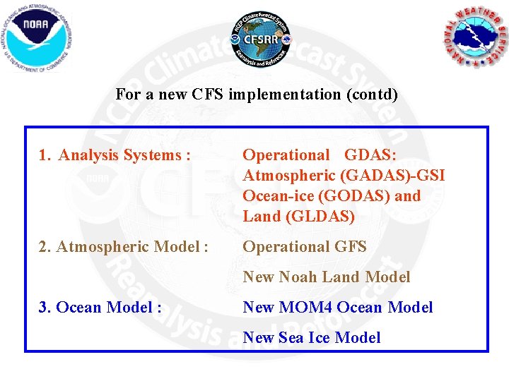
For a new CFS implementation (contd) 1. Analysis Systems : Operational GDAS: Atmospheric (GADAS)-GSI Ocean-ice (GODAS) and Land (GLDAS) 2. Atmospheric Model : Operational GFS New Noah Land Model 3. Ocean Model : New MOM 4 Ocean Model New Sea Ice Model

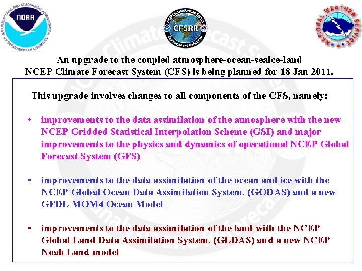
An upgrade to the coupled atmosphere-ocean-seaice-land NCEP Climate Forecast System (CFS) is being planned for 18 Jan 2011. This upgrade involves changes to all components of the CFS, namely: • improvements to the data assimilation of the atmosphere with the new NCEP Gridded Statistical Interpolation Scheme (GSI) and major improvements to the physics and dynamics of operational NCEP Global Forecast System (GFS) • improvements to the data assimilation of the ocean and ice with the NCEP Global Ocean Data Assimilation System, (GODAS) and a new GFDL MOM 4 Ocean Model • improvements to the data assimilation of the land with the NCEP Global Land Data Assimilation System, (GLDAS) and a new NCEP Noah Land model

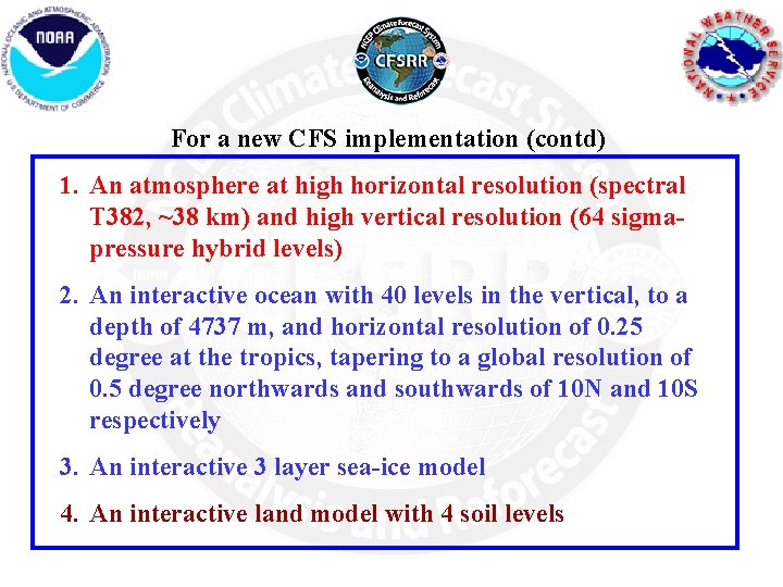
For a new CFS implementation (contd) 1. An atmosphere at high horizontal resolution (spectral T 382, ~38 km) and high vertical resolution (64 sigmapressure hybrid levels) 2. An interactive ocean with 40 levels in the vertical, to a depth of 4737 m, and horizontal resolution of 0. 25 degree at the tropics, tapering to a global resolution of 0. 5 degree northwards and southwards of 10 N and 10 S respectively 3. An interactive 3 layer sea-ice model 4. An interactive land model with 4 soil levels

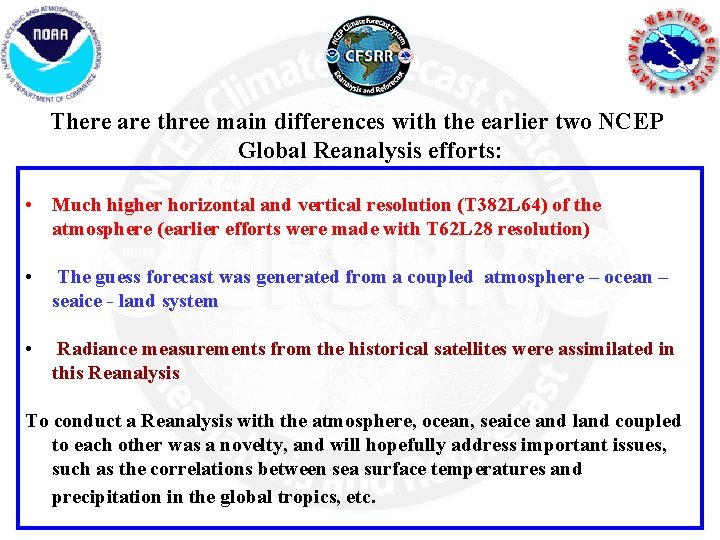
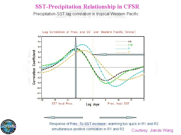
There are three main differences with the earlier two NCEP Global Reanalysis efforts: • Much higher horizontal and vertical resolution (T 382 L 64) of the atmosphere (earlier efforts were made with T 62 L 28 resolution) • The guess forecast was generated from a coupled atmosphere – ocean – seaice - land system • Radiance measurements from the historical satellites were assimilated in this Reanalysis To conduct a Reanalysis with the atmosphere, ocean, seaice and land coupled to each other was a novelty, and will hopefully address important issues, such as the correlations between sea surface temperatures and precipitation in the global tropics, etc.

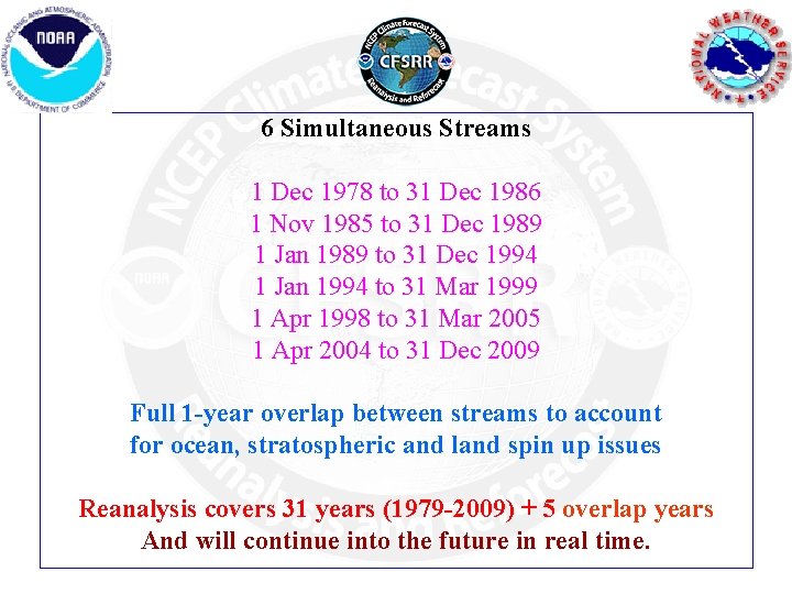
6 Simultaneous Streams 1 Dec 1978 to 31 Dec 1986 1 Nov 1985 to 31 Dec 1989 1 Jan 1989 to 31 Dec 1994 1 Jan 1994 to 31 Mar 1999 1 Apr 1998 to 31 Mar 2005 1 Apr 2004 to 31 Dec 2009 Full 1 -year overlap between streams to account for ocean, stratospheric and land spin up issues Reanalysis covers 31 years (1979 -2009) + 5 overlap years And will continue into the future in real time.

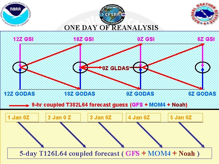
ONE DAY OF REANALYSIS 12 Z GSI 18 Z GSI 0 Z GSI 6 Z GSI 0 Z GODAS 6 Z GODAS 0 Z GLDAS 12 Z GODAS 18 Z GODAS 9 -hr coupled T 382 L 64 forecast guess (GFS + MOM 4 + Noah) 1 Jan 0 Z 2 Jan 0 Z 3 Jan 0 Z 4 Jan 0 Z 5 -day T 126 L 64 coupled forecast ( GFS + MOM 4 + Noah )

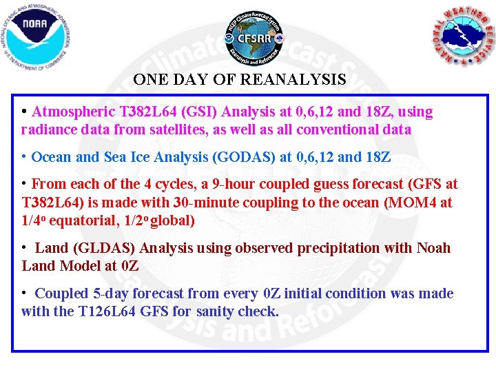
ONE DAY OF REANALYSIS • Atmospheric T 382 L 64 (GSI) Analysis at 0, 6, 12 and 18 Z, using radiance data from satellites, as well as all conventional data • Ocean and Sea Ice Analysis (GODAS) at 0, 6, 12 and 18 Z • From each of the 4 cycles, a 9 -hour coupled guess forecast (GFS at T 382 L 64) is made with 30 -minute coupling to the ocean (MOM 4 at 1/4 o equatorial, 1/2 o global) • Land (GLDAS) Analysis using observed precipitation with Noah Land Model at 0 Z • Coupled 5 -day forecast from every 0 Z initial condition was made with the T 126 L 64 GFS for sanity check.

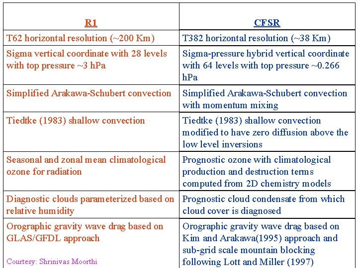
R 1 CFSR T 62 horizontal resolution (~200 Km) T 382 horizontal resolution (~38 Km) Sigma vertical coordinate with 28 levels with top pressure ~3 h. Pa Sigma-pressure hybrid vertical coordinate with 64 levels with top pressure ~0. 266 h. Pa Simplified Arakawa-Schubert convection with momentum mixing Tiedtke (1983) shallow convection modified to have zero diffusion above the low level inversions Seasonal and zonal mean climatological ozone for radiation Prognostic ozone with climatological production and destruction terms computed from 2 D chemistry models Diagnostic clouds parameterized based on Prognostic cloud condensate from which relative humidity cloud cover is diagnosed Orographic gravity wave drag based on GLAS/GFDL approach Courtesy: Shrinivas Moorthi Orographic gravity wave drag based on Kim and Arakawa(1995) approach and sub-grid scale mountain blocking following Lott and Miller (1997)

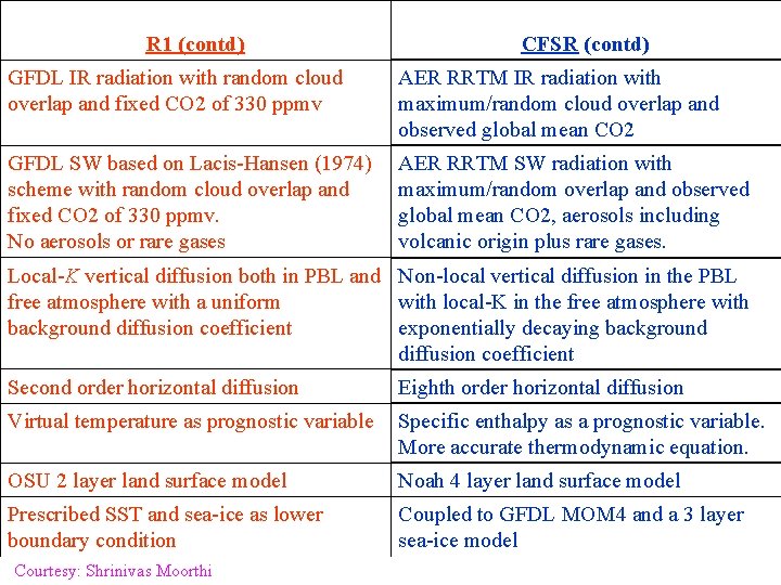
R 1 (contd) CFSR (contd) GFDL IR radiation with random cloud overlap and fixed CO 2 of 330 ppmv AER RRTM IR radiation with maximum/random cloud overlap and observed global mean CO 2 GFDL SW based on Lacis-Hansen (1974) scheme with random cloud overlap and fixed CO 2 of 330 ppmv. No aerosols or rare gases AER RRTM SW radiation with maximum/random overlap and observed global mean CO 2, aerosols including volcanic origin plus rare gases. Local-K vertical diffusion both in PBL and Non-local vertical diffusion in the PBL free atmosphere with a uniform with local-K in the free atmosphere with background diffusion coefficient exponentially decaying background diffusion coefficient Second order horizontal diffusion Eighth order horizontal diffusion Virtual temperature as prognostic variable Specific enthalpy as a prognostic variable. More accurate thermodynamic equation. OSU 2 layer land surface model Noah 4 layer land surface model Prescribed SST and sea-ice as lower boundary condition Coupled to GFDL MOM 4 and a 3 layer sea-ice model Courtesy: Shrinivas Moorthi

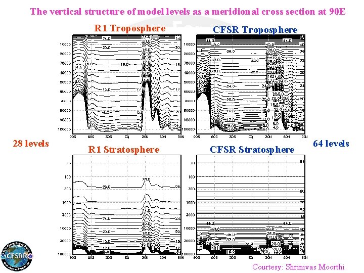
The vertical structure of model levels as a meridional cross section at 90 E R 1 Troposphere 28 levels R 1 Stratosphere CFSR Troposphere CFSR Stratosphere 64 levels Courtesy: Shrinivas Moorthi

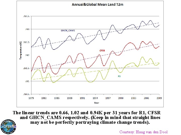
The linear trends are 0. 66, 1. 02 and 0. 94 K per 31 years for R 1, CFSR and GHCN_CAMS respectively. (Keep in mind that straight lines may not be perfectly portraying climate change trends). Courtesy: Huug van den Dool

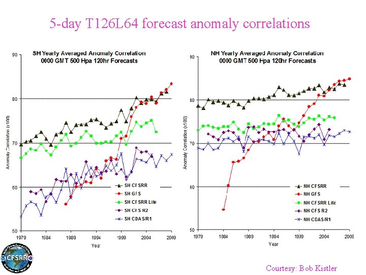
5 -day T 126 L 64 forecast anomaly correlations Courtesy: Bob Kistler

SST-Precipitation Relationship in CFSR Precipitation-SST lag correlation in tropical Western Pacific Response of Prec. To SST increase : warming too quick in R 1 and R 2 simultaneous positive correlation in R 1 and R 2 Courtesy: Jiande Wang

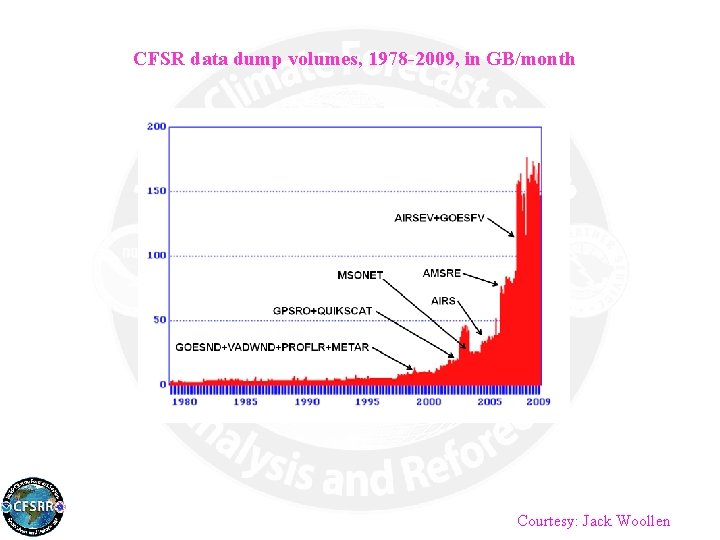
CFSR data dump volumes, 1978 -2009, in GB/month Courtesy: Jack Woollen

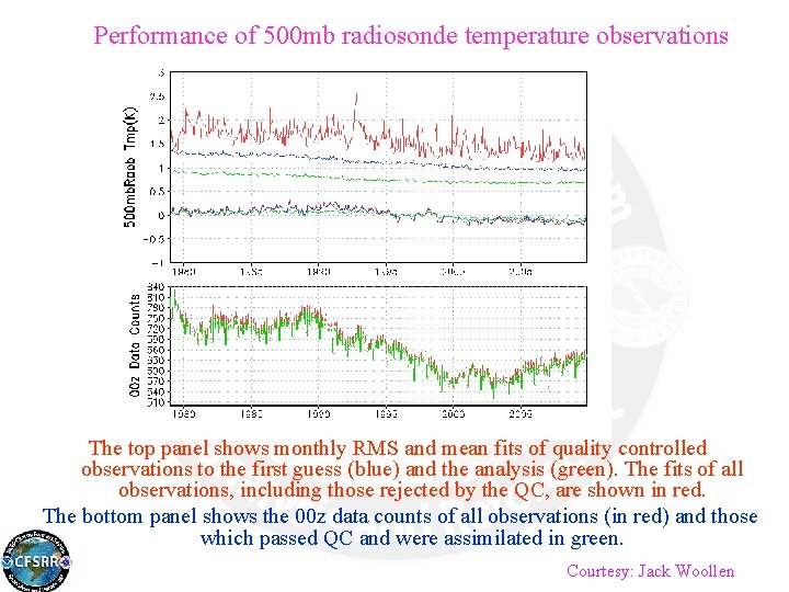
Performance of 500 mb radiosonde temperature observations The top panel shows monthly RMS and mean fits of quality controlled observations to the first guess (blue) and the analysis (green). The fits of all observations, including those rejected by the QC, are shown in red. The bottom panel shows the 00 z data counts of all observations (in red) and those which passed QC and were assimilated in green. Courtesy: Jack Woollen

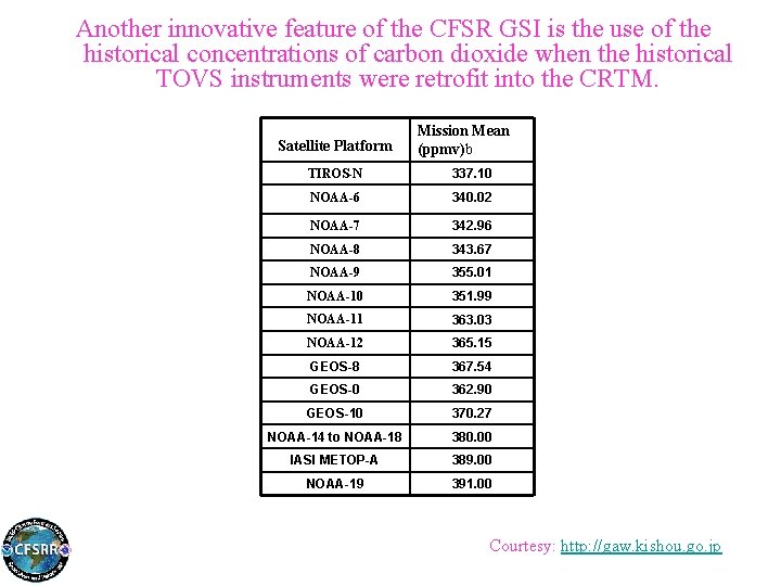
Another innovative feature of the CFSR GSI is the use of the historical concentrations of carbon dioxide when the historical TOVS instruments were retrofit into the CRTM. Satellite Platform Mission Mean (ppmv)b TIROS-N 337. 10 NOAA-6 340. 02 NOAA-7 342. 96 NOAA-8 343. 67 NOAA-9 355. 01 NOAA-10 351. 99 NOAA-11 363. 03 NOAA-12 365. 15 GEOS-8 367. 54 GEOS-0 362. 90 GEOS-10 370. 27 NOAA-14 to NOAA-18 380. 00 IASI METOP-A 389. 00 NOAA-19 391. 00 Courtesy: http: //gaw. kishou. go. jp

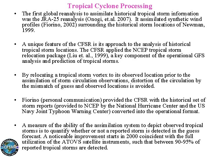
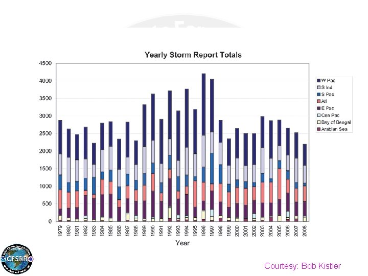
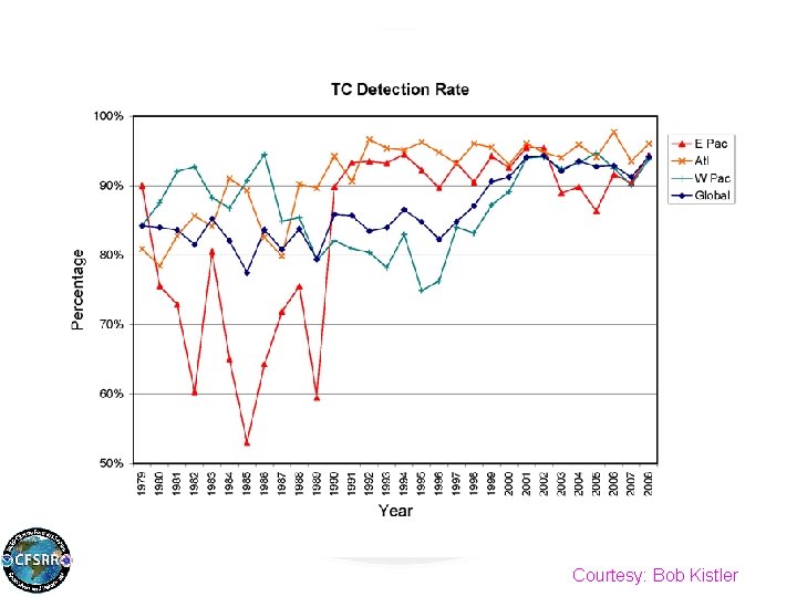
Tropical Cyclone Processing • The first global reanalysis to assimilate historical tropical storm information was the JRA-25 reanalysis (Onogi, et. al. 2007). It assimilated synthetic wind profiles (Fiorino, 2002) surrounding the historical storm locations of Newman, 1999. • A unique feature of the CFSR is its approach to the analysis of historical tropical storm locations. The CFSR applied the NCEP tropical storm relocation package (Liu et. al. , 1999), a key component of the operational GFS analysis and prediction of tropical storms. • By relocating a tropical storm vortex to its observed location prior to the assimilation of storm circulation observations, distortion of the circulation by the mismatch of guess and observed locations is avoided. • Fiorino (personal communication) provided the CFSR with the historical set of storm reports (provided to NCEP by the National Hurricane Center and the US Navy Joint Typhoon Warning Center) converted into the operational format. • A measure of the ability of the assimilation system to depict observed tropical storms is to quantify whether or not a reported storm is detected in the guess forecast. A noticeable improvement starts in 2000 coincident with the full utilization of the ATOVS satellite instruments, such that between 90 -95% of reported tropical storms are detected.

Courtesy: Bob Kistler

Courtesy: Bob Kistler

Transition to Real Time CFSR • The operational GSI had gone through several upgrades during the CFSR execution. In March 2009 a major addition was made to the CRTM to simulate the hyper-spectral channels of the IASI instrument, onboard the new ESA METOP satellite and NOAA-19 was added in Dec 2009. • In order to continue to meet the goal of providing the best available initial conditions to the CFS, in the absence of staff and resources to maintain the CFSR GSI into the future, it was decided to make the transition to the CDAS mode of CFSR in April 2008. • The operational GSI, present and future implementations, will replace the CFSR GSI, and the coupled prediction model will be “frozen” to that of the CFS v 2. • Historical observational datasets would be replaced with the operational data dumps.

THE OCEAN, SEA ICE AND COUPLER

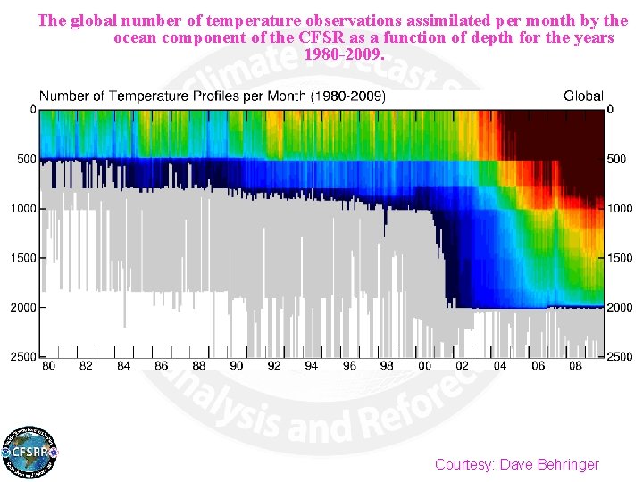
The global number of temperature observations assimilated per month by the ocean component of the CFSR as a function of depth for the years 1980 -2009. Courtesy: Dave Behringer

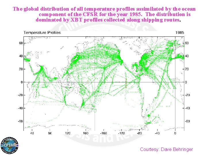
The global distribution of all temperature profiles assimilated by the ocean component of the CFSR for the year 1985. The distribution is dominated by XBT profiles collected along shipping routes. Courtesy: Dave Behringer

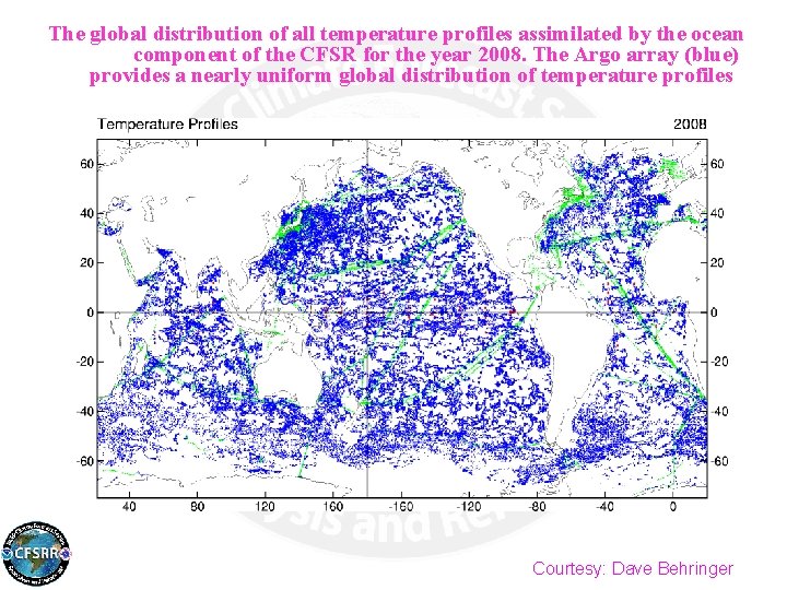
The global distribution of all temperature profiles assimilated by the ocean component of the CFSR for the year 2008. The Argo array (blue) provides a nearly uniform global distribution of temperature profiles Courtesy: Dave Behringer

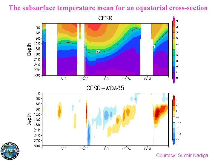
The subsurface temperature mean for an equatorial cross-section Courtesy: Sudhir Nadiga

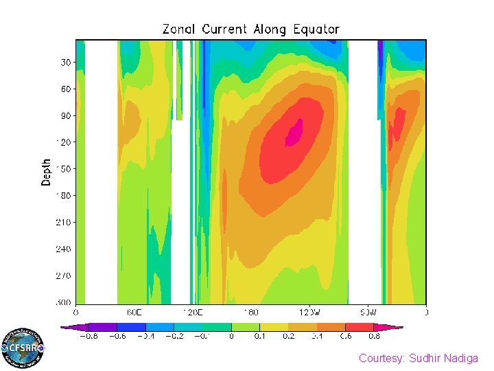
Courtesy: Sudhir Nadiga

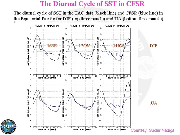
The Diurnal Cycle of SST in CFSR The diurnal cycle of SST in the TAO data (black line) and CFSR (blue line) in the Equatorial Pacific for DJF (top three panels) and JJA (bottom three panels). T 165 E 170 W 110 W DJF JJA Courtesy: Sudhir Nadiga

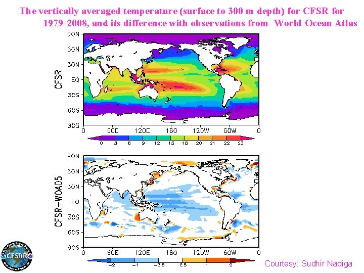
The vertically averaged temperature (surface to 300 m depth) for CFSR for 1979 -2008, and its difference with observations from World Ocean Atlas Courtesy: Sudhir Nadiga

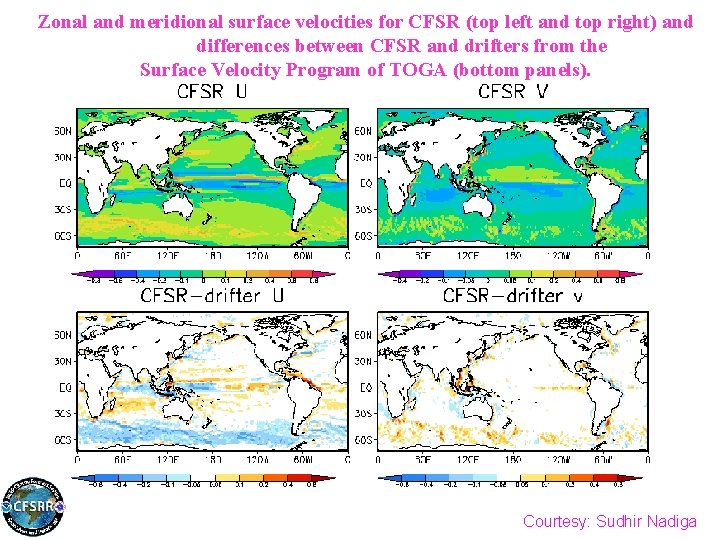
Zonal and meridional surface velocities for CFSR (top left and top right) and differences between CFSR and drifters from the Surface Velocity Program of TOGA (bottom panels). Courtesy: Sudhir Nadiga

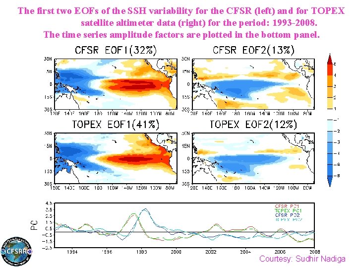
The first two EOFs of the SSH variability for the CFSR (left) and for TOPEX satellite altimeter data (right) for the period: 1993 -2008. The time series amplitude factors are plotted in the bottom panel. Courtesy: Sudhir Nadiga

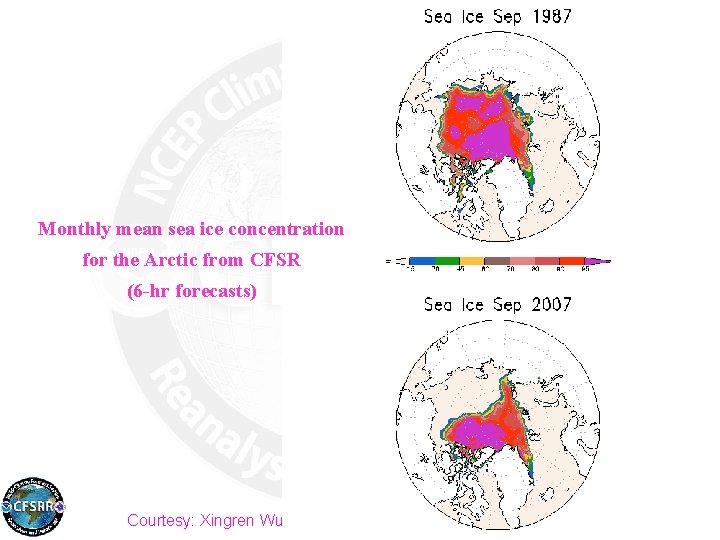
Monthly mean sea ice concentration for the Arctic from CFSR (6 -hr forecasts) Courtesy: Xingren Wu

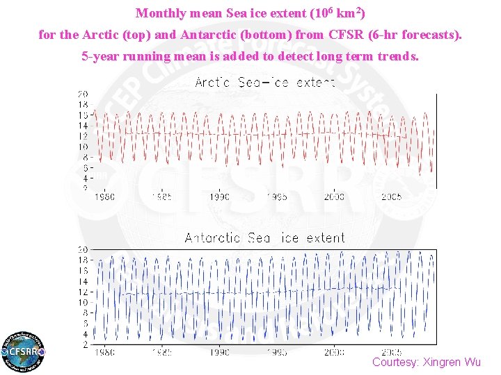
Monthly mean Sea ice extent (106 km 2) for the Arctic (top) and Antarctic (bottom) from CFSR (6 -hr forecasts). 5 -year running mean is added to detect long term trends. Courtesy: Xingren Wu

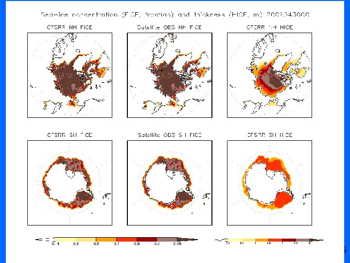
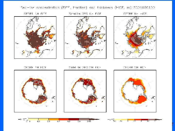
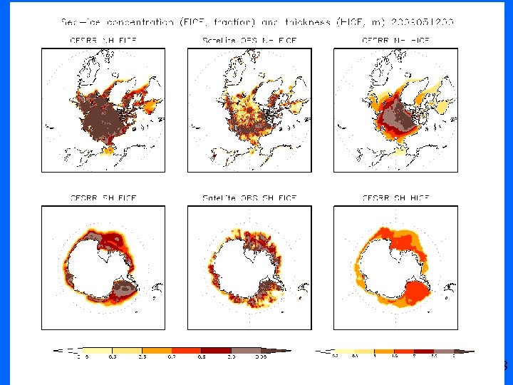
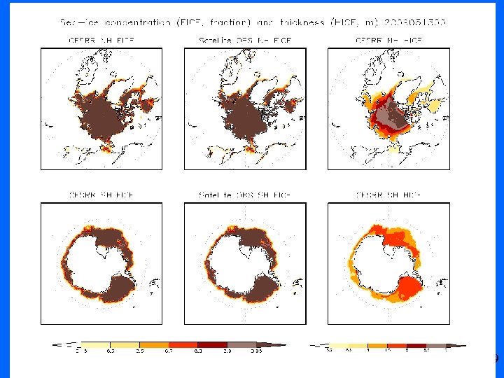
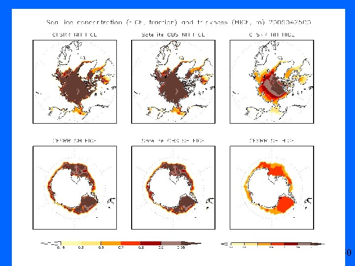
Problem for Sea-Ice Concentration in CFSRR for 2009: Due to the degradation of one of the DMSP F 15 sensor channels in February, and a problem from F 13 in early May 2009

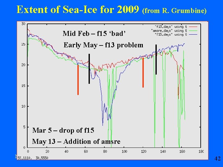
Extent of Sea-Ice for 2009 (from R. Grumbine) Mid Feb – f 15 ‘bad’ Early May – f 13 problem Mar 5 – drop of f 15 May 13 – Addition of amsre May 2009 Sea-Ice in CFSRR Climate Meeting: 9/2/2009 42

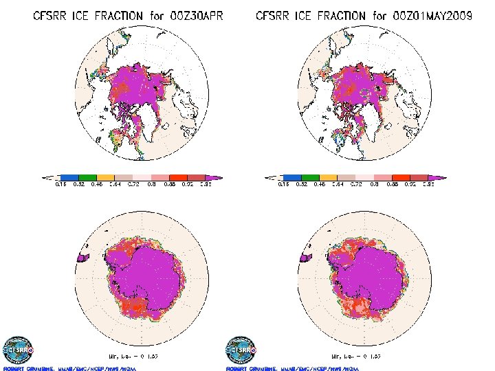
May 2009 Sea-Ice in CFSRR Climate Meeting: 9/2/2009 43

May 2009 Sea-Ice in CFSRR Climate Meeting: 9/2/2009 44

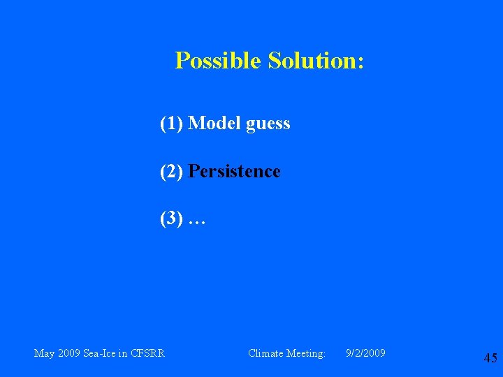
Possible Solution: (1) Model guess (2) Persistence (3) … May 2009 Sea-Ice in CFSRR Climate Meeting: 9/2/2009 45

May 2009 Sea-Ice in CFSRR Climate Meeting: 9/2/2009 46

May 2009 Sea-Ice in CFSRR Climate Meeting: 9/2/2009 47

May 2009 Sea-Ice in CFSRR Climate Meeting: 9/2/2009 48

May 2009 Sea-Ice in CFSRR Climate Meeting: 9/2/2009 49

May 2009 Sea-Ice in CFSRR Climate Meeting: 9/2/2009 50

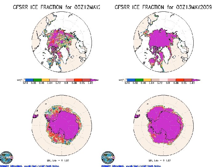
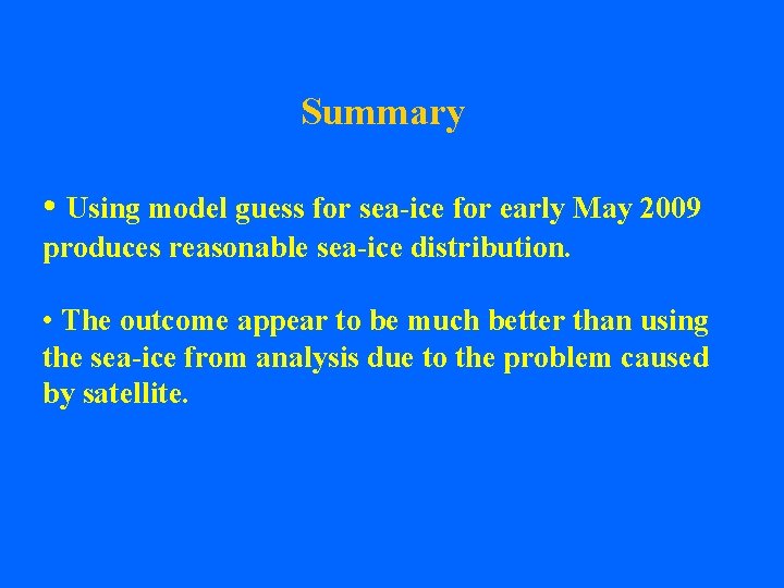
Summary • Using model guess for sea-ice for early May 2009 produces reasonable sea-ice distribution. • The outcome appear to be much better than using the sea-ice from analysis due to the problem caused by satellite.

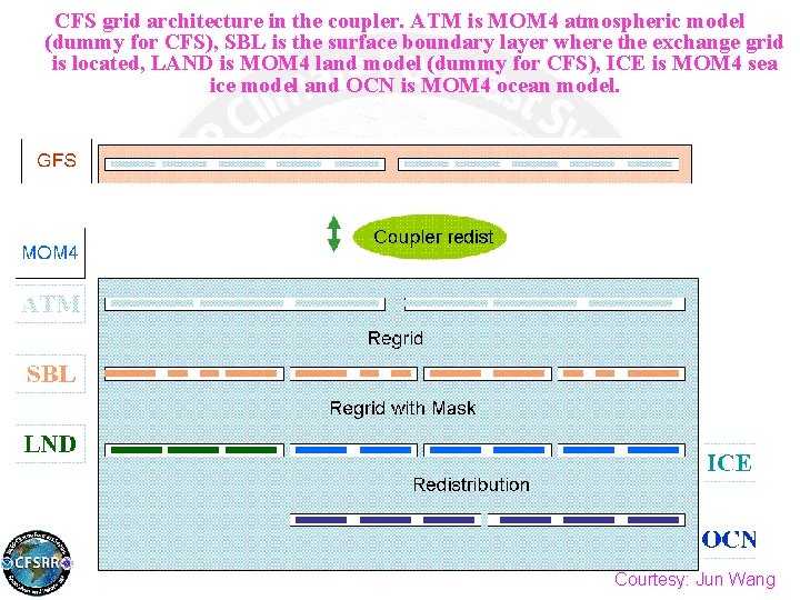
CFS grid architecture in the coupler. ATM is MOM 4 atmospheric model (dummy for CFS), SBL is the surface boundary layer where the exchange grid is located, LAND is MOM 4 land model (dummy for CFS), ICE is MOM 4 sea ice model and OCN is MOM 4 ocean model. Courtesy: Jun Wang

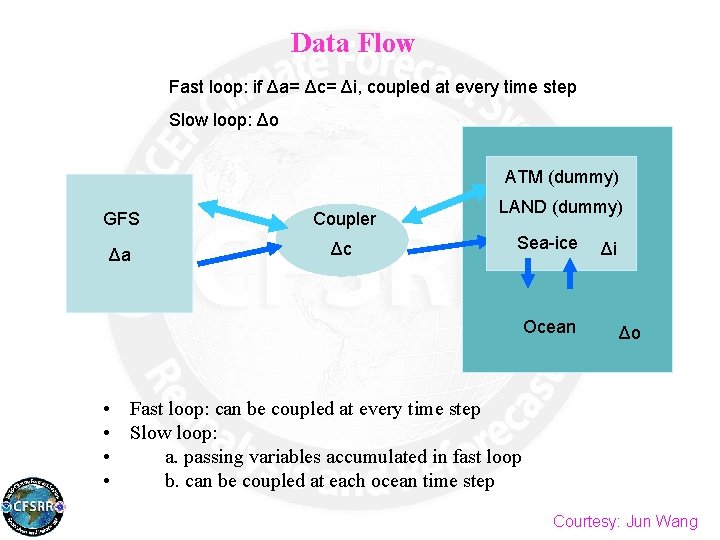
Data Flow Fast loop: if Δa= Δc= Δi, coupled at every time step Slow loop: Δo ATM (dummy) GFS Coupler Δa Δc LAND (dummy) Sea-ice Ocean Δi Δo • Fast loop: can be coupled at every time step • Slow loop: • a. passing variables accumulated in fast loop • b. can be coupled at each ocean time step Courtesy: Jun Wang

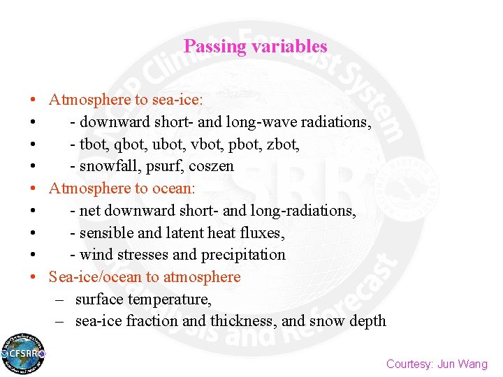
Passing variables • Atmosphere to sea-ice: • - downward short- and long-wave radiations, • - tbot, qbot, ubot, vbot, pbot, zbot, • - snowfall, psurf, coszen • Atmosphere to ocean: • - net downward short- and long-radiations, • - sensible and latent heat fluxes, • - wind stresses and precipitation • Sea-ice/ocean to atmosphere – surface temperature, – sea-ice fraction and thickness, and snow depth Courtesy: Jun Wang

THE SURFACE

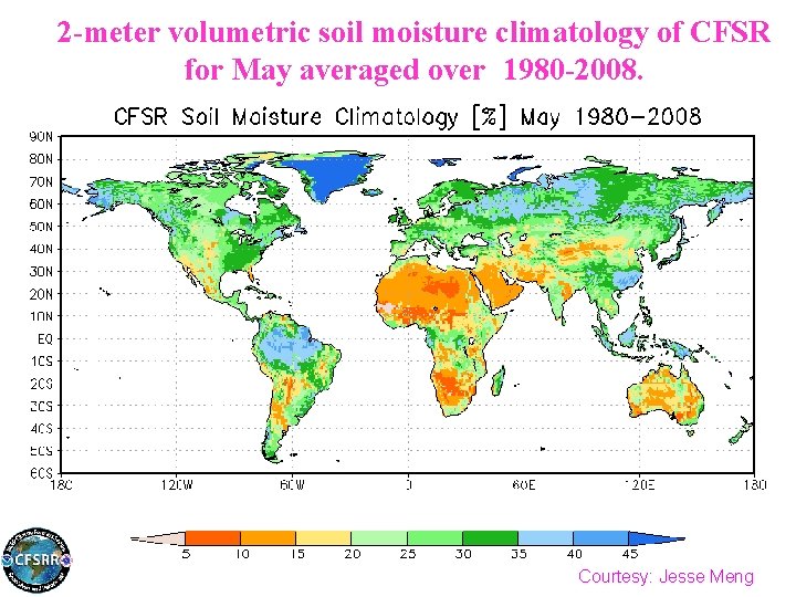
2 -meter volumetric soil moisture climatology of CFSR for May averaged over 1980 -2008. Courtesy: Jesse Meng

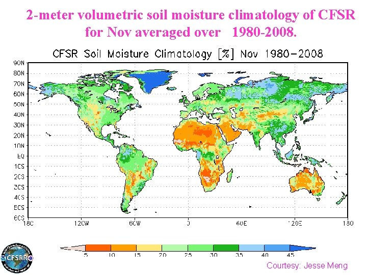
2 -meter volumetric soil moisture climatology of CFSR for Nov averaged over 1980 -2008. Courtesy: Jesse Meng

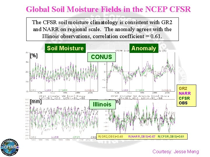
Global Soil Moisture Fields in the NCEP CFSR The CFSR soil moisture climatology is consistent with GR 2 and NARR on regional scale. The anomaly agrees with the Illinois observations, correlation coefficient = 0. 61. Soil Moisture [%] [mm] Anomaly [%] CONUS [mm] Illinois R(GR 2, OBS)=0. 48 GR 2 NARR CFSR OBS R(NARR, OBS)=0. 67 R(CFSR, OBS)=0. 61 Courtesy: Jesse Meng

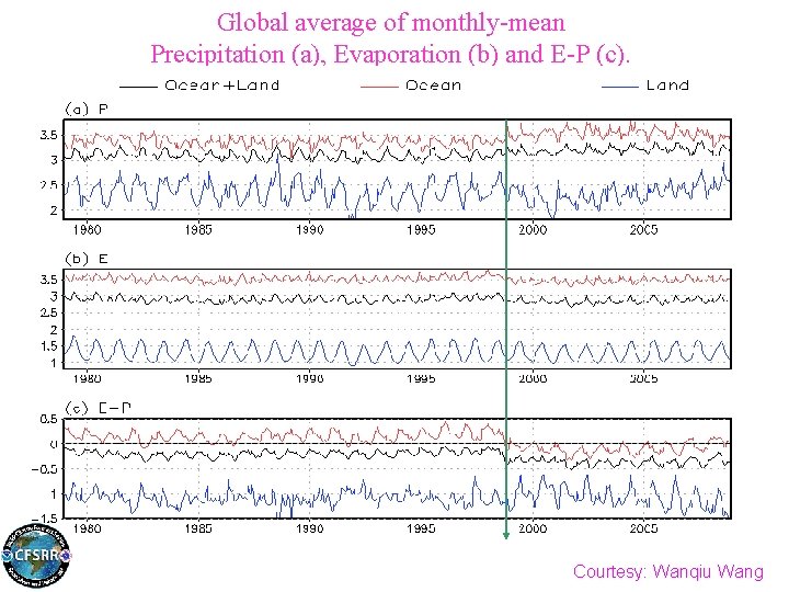
Global average of monthly-mean Precipitation (a), Evaporation (b) and E-P (c). Courtesy: Wanqiu Wang

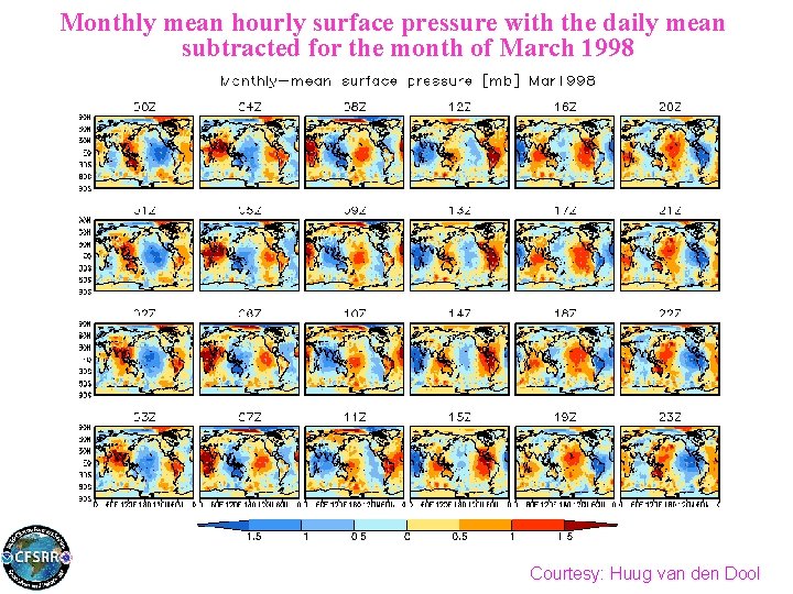
Monthly mean hourly surface pressure with the daily mean subtracted for the month of March 1998 Courtesy: Huug van den Dool

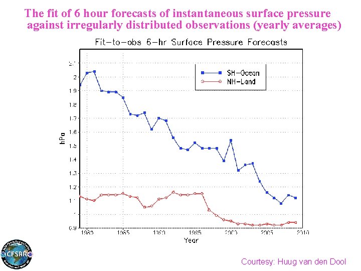
The fit of 6 hour forecasts of instantaneous surface pressure against irregularly distributed observations (yearly averages) Courtesy: Huug van den Dool

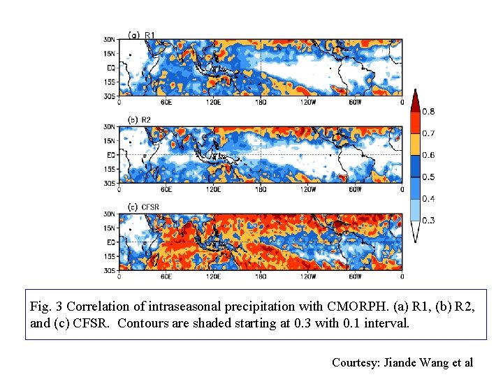
Fig. 3 Correlation of intraseasonal precipitation with CMORPH. (a) R 1, (b) R 2, and (c) CFSR. Contours are shaded starting at 0. 3 with 0. 1 interval. Courtesy: Jiande Wang et al

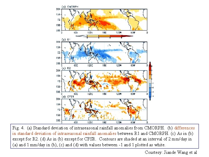
Fig. 4. (a) Standard deviation of intraseasonal rainfall anomalies from CMORPH. (b) differences in standard deviation of intraseasonal rainfall anomalies between R 1 and CMORPH. (c) As in (b) except for R 2. (d) As in (b) except for CFSR. Contours are shaded at an interval of 2 mm/day in (a) and 1 mm/day in (b), (c) and (d) with values between -1 and 1 plotted as white. Courtesy: Jiande Wang et al

Reference: Joyce, R. J. , J. E. Janowiak, P. A. Arkin, and P. Xie, 2004: CMORPH: A method that produces global precipitation estimates from passive microwave and infrared data at high spatial and temporal resolution. . J. Hydromet. , 5, 487 -503. CMORPH (CPC MORPHing technique) produces global precipitation analyses at very high spatial and temporal resolution. This technique uses precipitation estimates that have been derived from low orbiter satellite microwave observations exclusively, and whose features are transported via spatial propagation information that is obtained entirely from geostationary satellite IR data. At present we incorporate precipitation estimates derived from the passive microwaves aboard the DMSP 13, 14 & 15 (SSM/I), the NOAA-15, 16, 17 & 18 (AMSU-B), and AMSR-E and TMI aboard NASA's Aqua and TRMM spacecraft, respectively. These estimates are generated by algorithms of Ferraro (1997) for SSM/I, Ferraro et al. (2000) for AMSU-B and Kummerow et al. (2001) for TMI. Note that this technique is not a precipitation estimation algorithm but a means by which estimates from existing microwave rainfall algorithms can be combined. Therefore, this method is extremely flexible such that any precipitation estimates from any microwave satellite source can be incorporated.

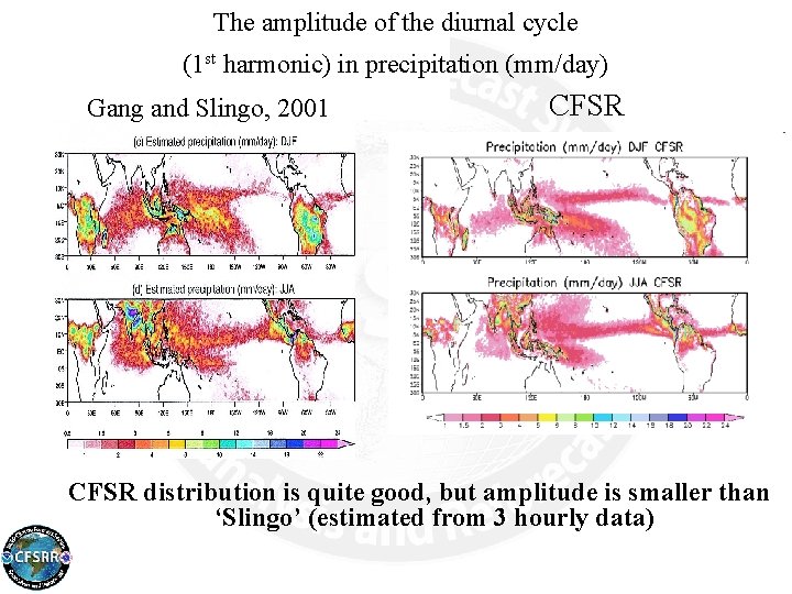
The amplitude of the diurnal cycle (1 st harmonic) in precipitation (mm/day) Gang and Slingo, 2001 CFSR distribution is quite good, but amplitude is smaller than ‘Slingo’ (estimated from 3 hourly data)

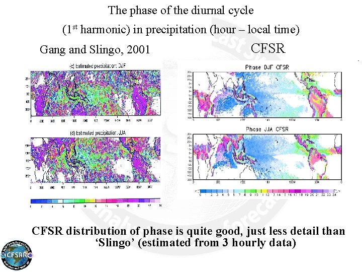
The phase of the diurnal cycle (1 st harmonic) in precipitation (hour – local time) Gang and Slingo, 2001 CFSR distribution of phase is quite good, just less detail than ‘Slingo’ (estimated from 3 hourly data)

THE STRATOSPHERE

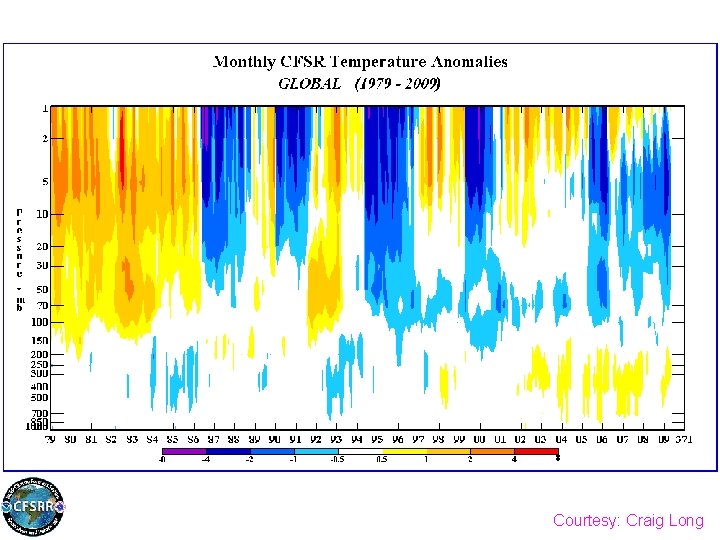
Courtesy: Craig Long

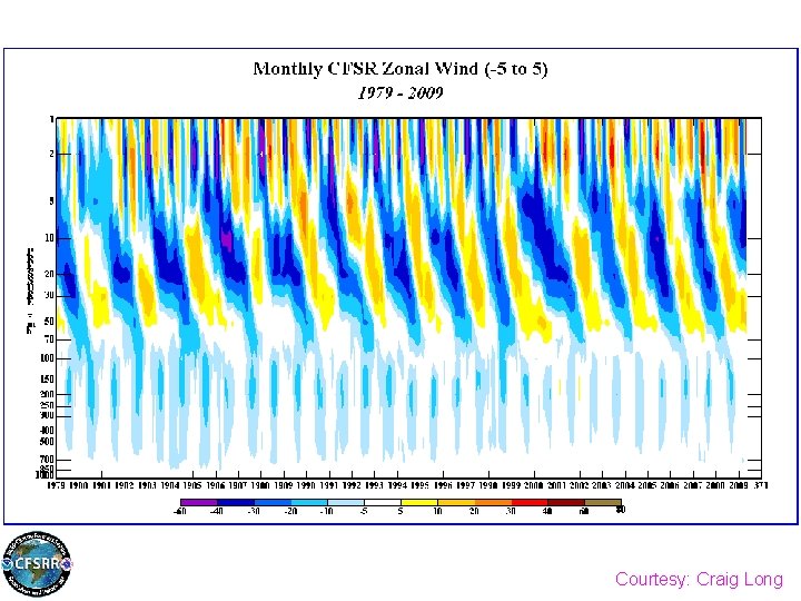
Courtesy: Craig Long

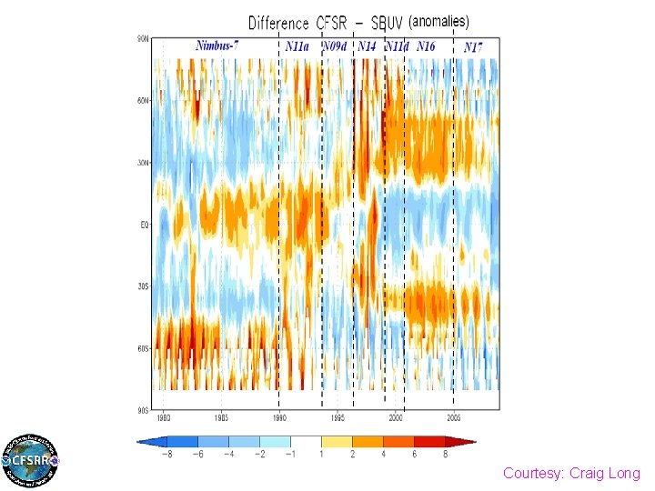
Courtesy: Craig Long

Future Plans • Immediately conduct CFSRL: a ‘light’ (with a reduced horizontal resolution of T 126) version of the reanalysis that was just completed. It will be done in a single stream to overcome the discontinuities found in the CFSR for the deep ocean, deep soil and the top of the atmosphere. It is possible that the CFSRL will be finished in 1 year, in time for CPC to use it when they change their climate normals to the last 30 -year period from 1981 -2010. • A final activity to be conducted when the Reforecast project is complete, is to apply the reanalysis system, as used here, to the historical period 1948 -1978. • The CFSR is the successor of R 2, and when extended back to 1948, will also be the successor of R 1. It is possible this will be done in one-stream ‘light’ mode.

THE CFSRR DREAM TEAM Jiande Sudhir Suru Xingren Patrick

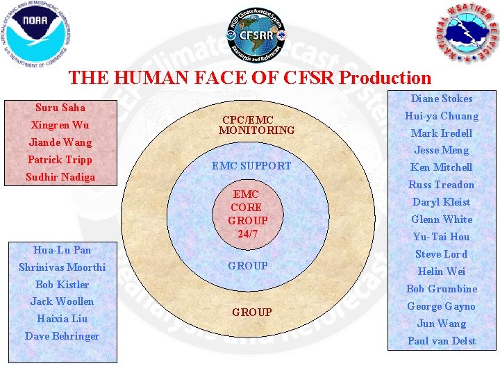
THE HUMAN FACE OF CFSR Production Diane Stokes Suru Saha Xingren Wu Jiande Wang Patrick Tripp Sudhir Nadiga CPC/EMC MONITORING EMC SUPPORT Hua-Lu Pan GROUP Bob Kistler Jack Woollen Haixia Liu Dave Behringer Mark Iredell Jesse Meng EMC CORE GROUP 24/7 Shrinivas Moorthi Hui-ya Chuang Ken Mitchell Russ Treadon Daryl Kleist Glenn White Yu-Tai Hou Steve Lord Helin Wei Bob Grumbine GROUP George Gayno Jun Wang Paul van Delst

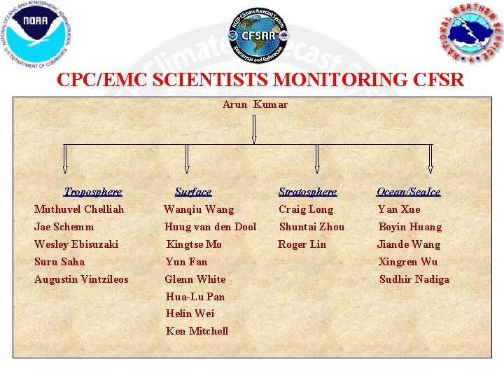
CPC/EMC SCIENTISTS MONITORING CFSR Arun Kumar Troposphere Surface Stratosphere Ocean/Sea. Ice Muthuvel Chelliah Wanqiu Wang Craig Long Yan Xue Jae Schemm Huug van den Dool Shuntai Zhou Boyin Huang Wesley Ebisuzaki Kingtse Mo Roger Lin Jiande Wang Suru Saha Yun Fan Xingren Wu Augustin Vintzileos Glenn White Sudhir Nadiga Hua-Lu Pan Helin Wei Ken Mitchell

AND NOW……. . THE SECOND ‘R’ IN

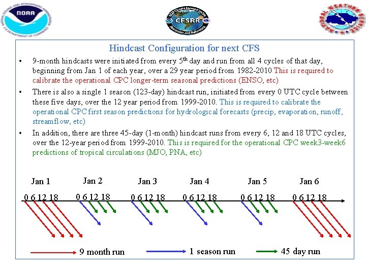
Hindcast Configuration for next CFS • • • 9 -month hindcasts were initiated from every 5 th day and run from all 4 cycles of that day, beginning from Jan 1 of each year, over a 29 year period from 1982 -2010 This is required to calibrate the operational CPC longer-term seasonal predictions (ENSO, etc) There is also a single 1 season (123 -day) hindcast run, initiated from every 0 UTC cycle between these five days, over the 12 year period from 1999 -2010. This is required to calibrate the operational CPC first season predictions for hydrological forecasts (precip, evaporation, runoff, streamflow, etc) In addition, there are three 45 -day (1 -month) hindcast runs from every 6, 12 and 18 UTC cycles, over the 12 -year period from 1999 -2010. This is required for the operational CPC week 3 -week 6 predictions of tropical circulations (MJO, PNA, etc) Jan 1 Jan 2 Jan 3 Jan 4 Jan 5 Jan 6 0 6 12 18 0 6 12 18 9 month run 1 season run 45 day run

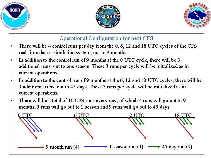
Operational Configuration for next CFS • • There will be 4 control runs per day from the 0, 6, 12 and 18 UTC cycles of the CFS real-time data assimilation system, out to 9 months. In addition to the control run of 9 months at the 0 UTC cycle, there will be 3 additional runs, out to one season. These 3 runs per cycle will be initialized as in current operations. In addition to the control run of 9 months at the 6, 12 and 18 UTC cycles, there will be 3 additional runs, out to 45 days. These 3 runs per cycle will be initialized as in current operations. There will be a total of 16 CFS runs every day, of which 4 runs will go out to 9 months, 3 runs will go out to 1 season and 9 runs will go out to 45 days. 0 UTC 6 UTC 9 month run (4) 12 UTC 18 UTC 1 season run (3) 45 day run (9)

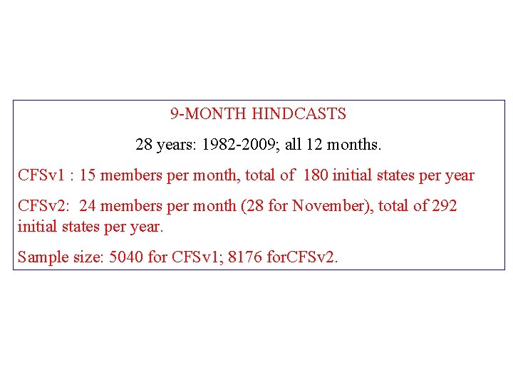
9 -MONTH HINDCASTS 28 years: 1982 -2009; all 12 months. CFSv 1 : 15 members per month, total of 180 initial states per year CFSv 2: 24 members per month (28 for November), total of 292 initial states per year. Sample size: 5040 for CFSv 1; 8176 for. CFSv 2.

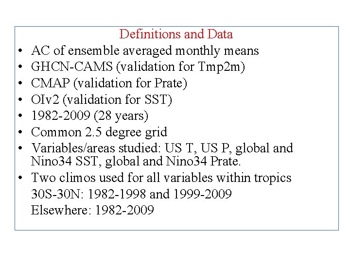
• • Definitions and Data AC of ensemble averaged monthly means GHCN-CAMS (validation for Tmp 2 m) CMAP (validation for Prate) OIv 2 (validation for SST) 1982 -2009 (28 years) Common 2. 5 degree grid Variables/areas studied: US T, US P, global and Nino 34 SST, global and Nino 34 Prate. Two climos used for all variables within tropics 30 S-30 N: 1982 -1998 and 1999 -2009 Elsewhere: 1982 -2009

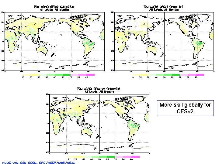
More skill globally for CFSv 2

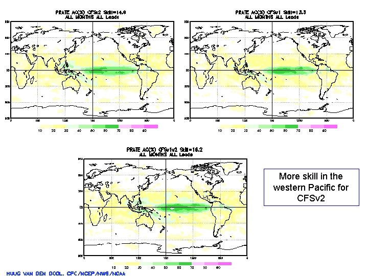
More skill in the western Pacific for CFSv 2

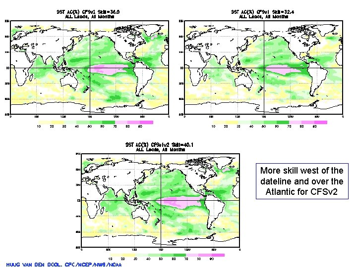
More skill west of the dateline and over the Atlantic for CFSv 2

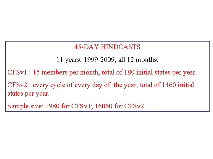
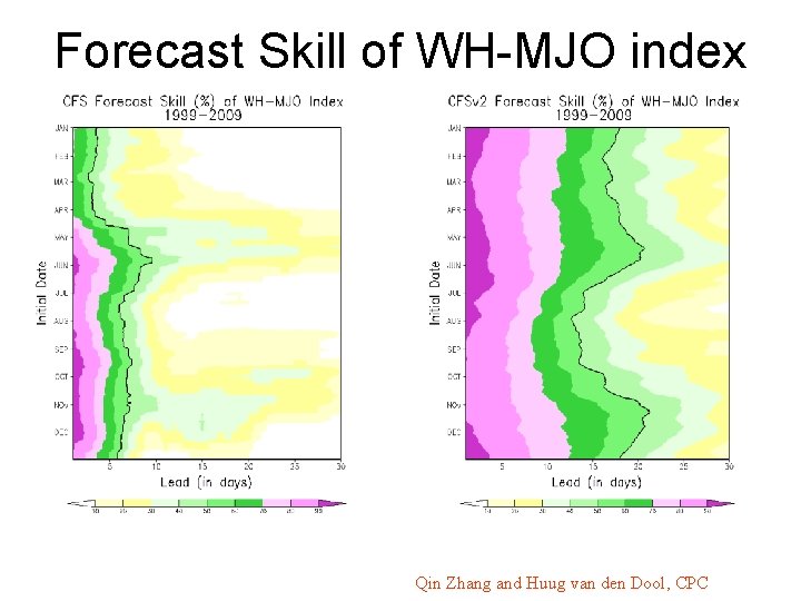
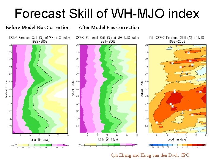
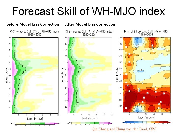
45 -DAY HINDCASTS 11 years: 1999 -2009; all 12 months. CFSv 1 : 15 members per month, total of 180 initial states per year CFSv 2: every cycle of every day of the year, total of 1460 initial states per year. Sample size: 1980 for CFSv 1; 16060 for CFSv 2.

Forecast Skill of WH-MJO index Qin Zhang and Huug van den Dool, CPC

Forecast Skill of WH-MJO index Before Model Bias Correction After Model Bias Correction Qin Zhang and Huug van den Dool, CPC

Forecast Skill of WH-MJO index Before Model Bias Correction After Model Bias Correction Qin Zhang and Huug van den Dool, CPC

DATA DESCRIPTION

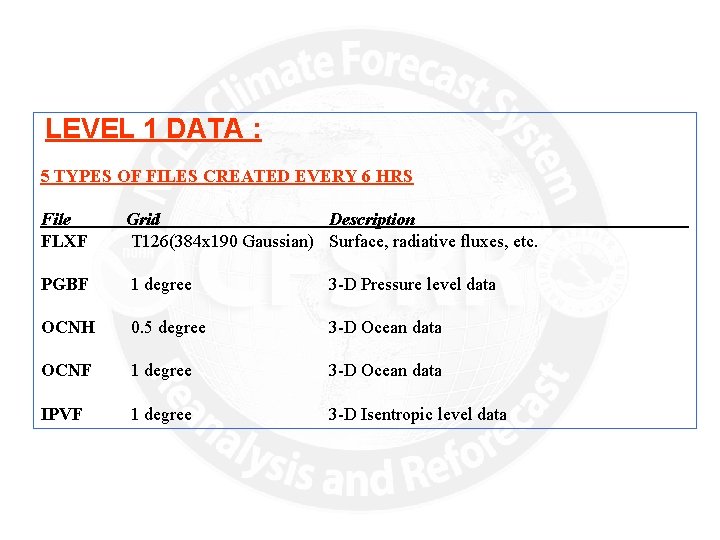
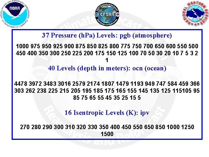
LEVEL 1 DATA : 5 TYPES OF FILES CREATED EVERY 6 HRS File FLXF Grid Description T 126(384 x 190 Gaussian) Surface, radiative fluxes, etc. PGBF 1 degree 3 -D Pressure level data OCNH 0. 5 degree 3 -D Ocean data OCNF 1 degree 3 -D Ocean data IPVF 1 degree 3 -D Isentropic level data

37 Pressure (h. Pa) Levels: pgb (atmosphere) 1000 975 950 925 900 875 850 825 800 775 750 700 650 600 550 500 450 400 350 300 250 225 200 175 150 125 100 70 50 30 20 10 7 5 3 2 1 40 Levels (depth in meters): ocn (ocean) 4478 3972 3483 3016 2579 2174 1807 1479 1193 949 747 584 459 366 303 262 238 225 215 205 195 185 175 165 155 145 135 125 115105 95 85 75 65 55 45 35 25 15 5 16 Isentropic Levels (K): ipv 270 280 290 300 310 320 330 350 400 450 550 650 850 1000 1250 1500

CONTENTS OF IPV FILES • LAPRtht 16 ** (profile) Lapse rate [K/m] • MNTSFtht 16 ** (profile) Montgomery stream function [m^2/s^2] • PRESsfc 0 ** (surface) Pressure [Pa] • PVORTtht 16 ** (profile) Pot. vorticity [km^2/kg/s] • RHtht 16 ** (profile) Relative humidity [%] • TMPsfc 0 ** (surface) Temp. [K] • TMPtht 16 ** (profile) Temp. [K] • UGRDtht 16 ** (profile) u wind [m/s] • VGRDtht 16 ** (profile) v wind [m/s] • VVELtht 16 ** (profile) Pressure vertical velocity [Pa/s]

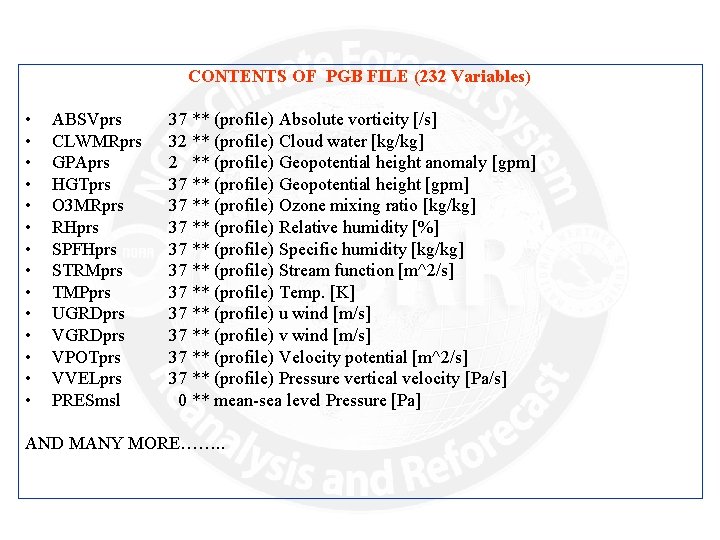
CONTENTS OF PGB FILE (232 Variables) • • • • ABSVprs CLWMRprs GPAprs HGTprs O 3 MRprs RHprs SPFHprs STRMprs TMPprs UGRDprs VPOTprs VVELprs PRESmsl 37 ** (profile) Absolute vorticity [/s] 32 ** (profile) Cloud water [kg/kg] 2 ** (profile) Geopotential height anomaly [gpm] 37 ** (profile) Geopotential height [gpm] 37 ** (profile) Ozone mixing ratio [kg/kg] 37 ** (profile) Relative humidity [%] 37 ** (profile) Specific humidity [kg/kg] 37 ** (profile) Stream function [m^2/s] 37 ** (profile) Temp. [K] 37 ** (profile) u wind [m/s] 37 ** (profile) v wind [m/s] 37 ** (profile) Velocity potential [m^2/s] 37 ** (profile) Pressure vertical velocity [Pa/s] 0 ** mean-sea level Pressure [Pa] AND MANY MORE……. .

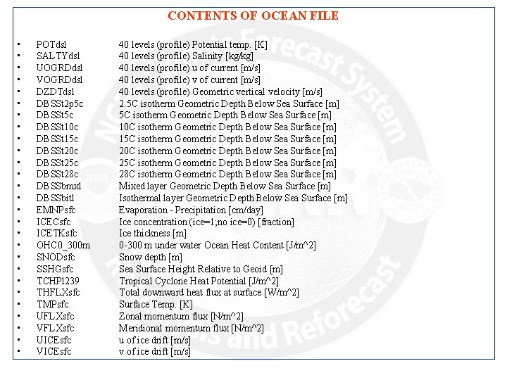
CONTENTS OF OCEAN FILE • • • • • • • POTdsl SALTYdsl UOGRDdsl VOGRDdsl DZDTdsl DBSSt 2 p 5 c DBSSt 10 c DBSSt 15 c DBSSt 20 c DBSSt 25 c DBSSt 28 c DBSSbmxl DBSSbitl EMNPsfc ICECsfc ICETKsfc OHC 0_300 m SNODsfc SSHGsfc TCHPl 239 THFLXsfc TMPsfc UFLXsfc VFLXsfc UICEsfc VICEsfc 40 levels (profile) Potential temp. [K] 40 levels (profile) Salinity [kg/kg] 40 levels (profile) u of current [m/s] 40 levels (profile) v of current [m/s] 40 levels (profile) Geometric vertical velocity [m/s] 2. 5 C isotherm Geometric Depth Below Sea Surface [m] 10 C isotherm Geometric Depth Below Sea Surface [m] 15 C isotherm Geometric Depth Below Sea Surface [m] 20 C isotherm Geometric Depth Below Sea Surface [m] 25 C isotherm Geometric Depth Below Sea Surface [m] 28 C isotherm Geometric Depth Below Sea Surface [m] Mixed layer Geometric Depth Below Sea Surface [m] Isothermal layer Geometric Depth Below Sea Surface [m] Evaporation - Precipitation [cm/day] Ice concentration (ice=1; no ice=0) [fraction] Ice thickness [m] 0 -300 m under water Ocean Heat Content [J/m^2] Snow depth [m] Sea Surface Height Relative to Geoid [m] Tropical Cyclone Heat Potential [J/m^2] Total downward heat flux at surface [W/m^2] Surface Temp. [K] Zonal momentum flux [N/m^2] Meridional momentum flux [N/m^2] u of ice drift [m/s] v of ice drift [m/s]

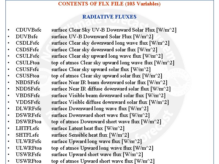
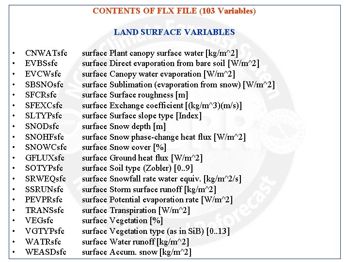
CONTENTS OF FLX FILE (103 Variables) RADIATIVE FLUXES • • • • • • CDUVBsfc CSDLFsfc CSDSFsfc CSULFtoa CSUSFsfc CSUSFtoa NBDSFsfc NDDSFsfc VBDSFsfc VDDSFsfc DLWRFsfc DSWRFtoa LHTFLsfc SHTFLsfc ULWRFtoa USWRFsfc USWRFtoa surface Clear Sky UV-B Downward Solar Flux [W/m^2] surface Clear sky downward long wave flux [W/m^2] surface Clear sky downward solar flux [W/m^2] surface Clear sky upward long wave flux [W/m^2] top of atmos Clear sky upward long wave flux [W/m^2] surface Clear sky upward solar flux [W/m^2] top of atmos Clear sky upward solar flux [W/m^2] surface Near IR beam downward solar flux [W/m^2] surface Near IR diffuse downward solar flux [W/m^2] surface Visible beam downward solar flux [W/m^2] surface Visible diffuse downward solar flux [W/m^2] surface Downward long wave flux [W/m^2] surface Downward short wave flux [W/m^2] top of atmos Downward short wave flux [W/m^2] surface Latent heat flux [W/m^2] surface Sensible heat flux [W/m^2] surface Upward long wave flux [W/m^2] top of atmos Upward long wave flux [W/m^2] surface Upward short wave flux [W/m^2] top of atmos Upward short wave flux [W/m^2]

CONTENTS OF FLX FILE (103 Variables) LAND SURFACE VARIABLES • • • • • CNWATsfc EVBSsfc EVCWsfc SBSNOsfc SFCRsfc SFEXCsfc SLTYPsfc SNODsfc SNOHFsfc SNOWCsfc GFLUXsfc SOTYPsfc SRWEQsfc SSRUNsfc PEVPRsfc TRANSsfc VEGsfc VGTYPsfc WATRsfc WEASDsfc surface Plant canopy surface water [kg/m^2] surface Direct evaporation from bare soil [W/m^2] surface Canopy water evaporation [W/m^2] surface Sublimation (evaporation from snow) [W/m^2] surface Surface roughness [m] surface Exchange coefficient [(kg/m^3)(m/s)] surface Surface slope type [Index] surface Snow depth [m] surface Snow phase-change heat flux [W/m^2] surface Snow cover [%] surface Ground heat flux [W/m^2] surface Soil type (Zobler) [0. . 9] surface Snowfall rate water equiv. [kg/m^2/s] surface Storm surface runoff [kg/m^2] surface Potential evaporation rate [W/m^2] surface Transpiration [W/m^2] surface Vegetation [%] surface Vegetation type (as in Si. B) [0. . 13] surface Water runoff [kg/m^2] surface Accum. snow [kg/m^2]

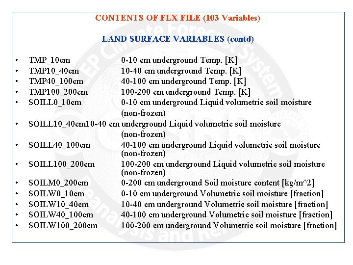
CONTENTS OF FLX FILE (103 Variables) LAND SURFACE VARIABLES (contd) • • • • TMP_10 cm TMP 10_40 cm TMP 40_100 cm TMP 100_200 cm SOILL 0_10 cm 0 -10 cm underground Temp. [K] 10 -40 cm underground Temp. [K] 40 -100 cm underground Temp. [K] 100 -200 cm underground Temp. [K] 0 -10 cm underground Liquid volumetric soil moisture (non-frozen) SOILL 10_40 cm 10 -40 cm underground Liquid volumetric soil moisture (non-frozen) SOILL 40_100 cm 40 -100 cm underground Liquid volumetric soil moisture (non-frozen) SOILL 100_200 cm 100 -200 cm underground Liquid volumetric soil moisture (non-frozen) SOILM 0_200 cm 0 -200 cm underground Soil moisture content [kg/m^2] SOILW 0_10 cm 0 -10 cm underground Volumetric soil moisture [fraction] SOILW 10_40 cm 10 -40 cm underground Volumetric soil moisture [fraction] SOILW 40_100 cm 40 -100 cm underground Volumetric soil moisture [fraction] SOILW 100_200 cm 100 -200 cm underground Volumetric soil moisture [fraction]

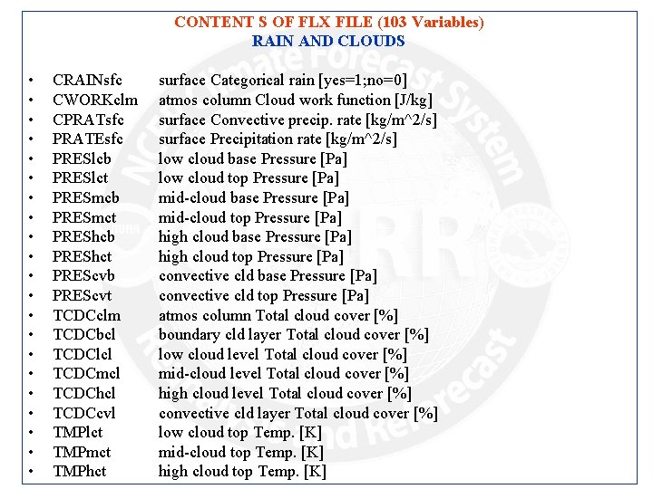
CONTENT S OF FLX FILE (103 Variables) RAIN AND CLOUDS • • • • • • CRAINsfc CWORKclm CPRATsfc PRATEsfc PRESlcb PRESlct PRESmcb PRESmct PREShcb PREShct PREScvb PREScvt TCDCclm TCDCbcl TCDClcl TCDCmcl TCDChcl TCDCcvl TMPlct TMPmct TMPhct surface Categorical rain [yes=1; no=0] atmos column Cloud work function [J/kg] surface Convective precip. rate [kg/m^2/s] surface Precipitation rate [kg/m^2/s] low cloud base Pressure [Pa] low cloud top Pressure [Pa] mid-cloud base Pressure [Pa] mid-cloud top Pressure [Pa] high cloud base Pressure [Pa] high cloud top Pressure [Pa] convective cld base Pressure [Pa] convective cld top Pressure [Pa] atmos column Total cloud cover [%] boundary cld layer Total cloud cover [%] low cloud level Total cloud cover [%] mid-cloud level Total cloud cover [%] high cloud level Total cloud cover [%] convective cld layer Total cloud cover [%] low cloud top Temp. [K] mid-cloud top Temp. [K] high cloud top Temp. [K]

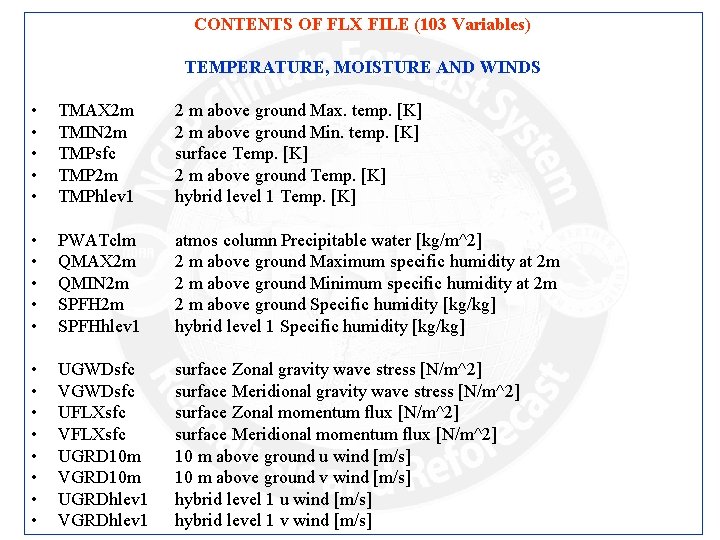
CONTENTS OF FLX FILE (103 Variables) TEMPERATURE, MOISTURE AND WINDS • • • TMAX 2 m TMIN 2 m TMPsfc TMP 2 m TMPhlev 1 2 m above ground Max. temp. [K] 2 m above ground Min. temp. [K] surface Temp. [K] 2 m above ground Temp. [K] hybrid level 1 Temp. [K] • • • PWATclm QMAX 2 m QMIN 2 m SPFHhlev 1 atmos column Precipitable water [kg/m^2] 2 m above ground Maximum specific humidity at 2 m 2 m above ground Minimum specific humidity at 2 m 2 m above ground Specific humidity [kg/kg] hybrid level 1 Specific humidity [kg/kg] • • UGWDsfc VGWDsfc UFLXsfc VFLXsfc UGRD 10 m VGRD 10 m UGRDhlev 1 VGRDhlev 1 surface Zonal gravity wave stress [N/m^2] surface Meridional gravity wave stress [N/m^2] surface Zonal momentum flux [N/m^2] surface Meridional momentum flux [N/m^2] 10 m above ground u wind [m/s] 10 m above ground v wind [m/s] hybrid level 1 u wind [m/s] hybrid level 1 v wind [m/s]

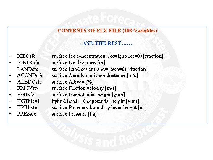
CONTENTS OF FLX FILE (103 Variables) AND THE REST…… • • • ICECsfc ICETKsfc LANDsfc ACONDsfc ALBDOsfc FRICVsfc HGThlev 1 HPBLsfc PRESsfc surface Ice concentration (ice=1; no ice=0) [fraction] surface Ice thickness [m] surface Land cover (land=1; sea=0) [fraction] surface Aerodynamic conductance [m/s] surface Albedo [%] surface Friction velocity [m/s] surface Geopotential height [gpm] hybrid level 1 Geopotential height [gpm] surface Planetary boundary layer height [m] surface Pressure [Pa]

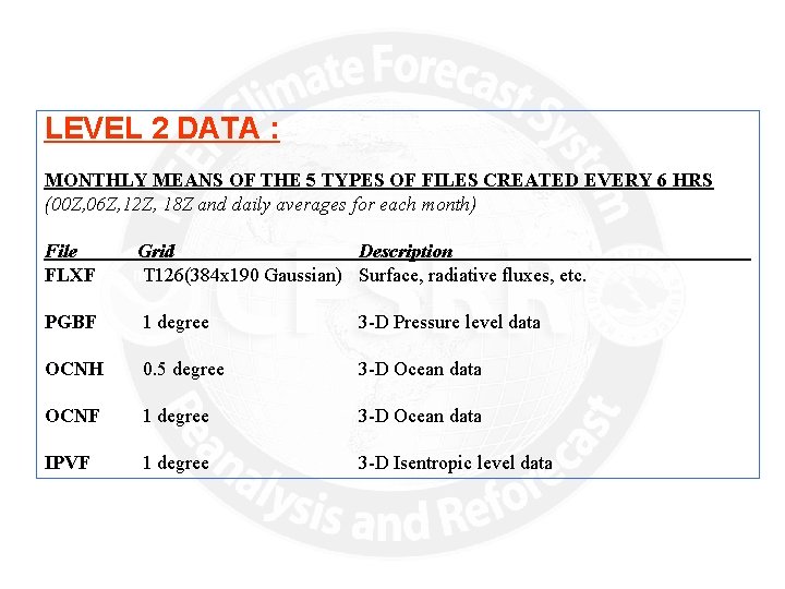
LEVEL 2 DATA : MONTHLY MEANS OF THE 5 TYPES OF FILES CREATED EVERY 6 HRS (00 Z, 06 Z, 12 Z, 18 Z and daily averages for each month) File FLXF Grid Description T 126(384 x 190 Gaussian) Surface, radiative fluxes, etc. PGBF 1 degree 3 -D Pressure level data OCNH 0. 5 degree 3 -D Ocean data OCNF 1 degree 3 -D Ocean data IPVF 1 degree 3 -D Isentropic level data

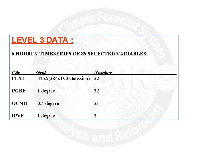
LEVEL 3 DATA : 6 HOURLY TIMESERIES OF 88 SELECTED VARIABLES File FLXF Grid Number T 126(384 x 190 Gaussian) 32 PGBF 1 degree 32 OCNH 0. 5 degree 21 IPVF 1 degree 3

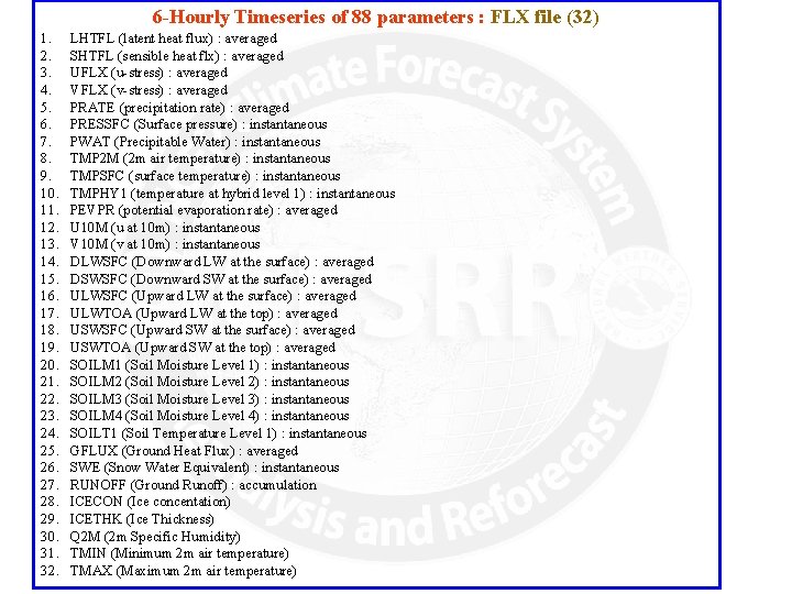
6 -Hourly Timeseries of 88 parameters : FLX file (32) 1. 2. 3. 4. 5. 6. 7. 8. 9. 10. 11. 12. 13. 14. 15. 16. 17. 18. 19. 20. 21. 22. 23. 24. 25. 26. 27. 28. 29. 30. 31. 32. LHTFL (latent heat flux) : averaged SHTFL (sensible heat flx) : averaged UFLX (u-stress) : averaged VFLX (v-stress) : averaged PRATE (precipitation rate) : averaged PRESSFC (Surface pressure) : instantaneous PWAT (Precipitable Water) : instantaneous TMP 2 M (2 m air temperature) : instantaneous TMPSFC (surface temperature) : instantaneous TMPHY 1 (temperature at hybrid level 1) : instantaneous PEVPR (potential evaporation rate) : averaged U 10 M (u at 10 m) : instantaneous V 10 M (v at 10 m) : instantaneous DLWSFC (Downward LW at the surface) : averaged DSWSFC (Downward SW at the surface) : averaged ULWSFC (Upward LW at the surface) : averaged ULWTOA (Upward LW at the top) : averaged USWSFC (Upward SW at the surface) : averaged USWTOA (Upward SW at the top) : averaged SOILM 1 (Soil Moisture Level 1) : instantaneous SOILM 2 (Soil Moisture Level 2) : instantaneous SOILM 3 (Soil Moisture Level 3) : instantaneous SOILM 4 (Soil Moisture Level 4) : instantaneous SOILT 1 (Soil Temperature Level 1) : instantaneous GFLUX (Ground Heat Flux) : averaged SWE (Snow Water Equivalent) : instantaneous RUNOFF (Ground Runoff) : accumulation ICECON (Ice concentation) ICETHK (Ice Thickness) Q 2 M (2 m Specific Humidity) TMIN (Minimum 2 m air temperature) TMAX (Maximum 2 m air temperature)

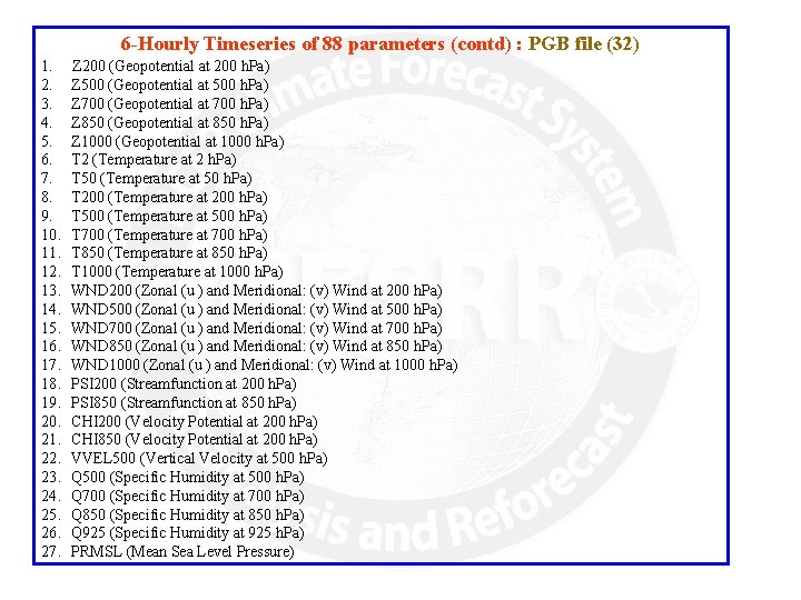
6 -Hourly Timeseries of 88 parameters (contd) : PGB file (32) 1. 2. 3. 4. 5. 6. 7. 8. 9. 10. 11. 12. 13. 14. 15. 16. 17. 18. 19. 20. 21. 22. 23. 24. 25. 26. 27. Z 200 (Geopotential at 200 h. Pa) Z 500 (Geopotential at 500 h. Pa) Z 700 (Geopotential at 700 h. Pa) Z 850 (Geopotential at 850 h. Pa) Z 1000 (Geopotential at 1000 h. Pa) T 2 (Temperature at 2 h. Pa) T 50 (Temperature at 50 h. Pa) T 200 (Temperature at 200 h. Pa) T 500 (Temperature at 500 h. Pa) T 700 (Temperature at 700 h. Pa) T 850 (Temperature at 850 h. Pa) T 1000 (Temperature at 1000 h. Pa) WND 200 (Zonal (u ) and Meridional: (v) Wind at 200 h. Pa) WND 500 (Zonal (u ) and Meridional: (v) Wind at 500 h. Pa) WND 700 (Zonal (u ) and Meridional: (v) Wind at 700 h. Pa) WND 850 (Zonal (u ) and Meridional: (v) Wind at 850 h. Pa) WND 1000 (Zonal (u ) and Meridional: (v) Wind at 1000 h. Pa) PSI 200 (Streamfunction at 200 h. Pa) PSI 850 (Streamfunction at 850 h. Pa) CHI 200 (Velocity Potential at 200 h. Pa) CHI 850 (Velocity Potential at 200 h. Pa) VVEL 500 (Vertical Velocity at 500 h. Pa) Q 500 (Specific Humidity at 500 h. Pa) Q 700 (Specific Humidity at 700 h. Pa) Q 850 (Specific Humidity at 850 h. Pa) Q 925 (Specific Humidity at 925 h. Pa) PRMSL (Mean Sea Level Pressure)

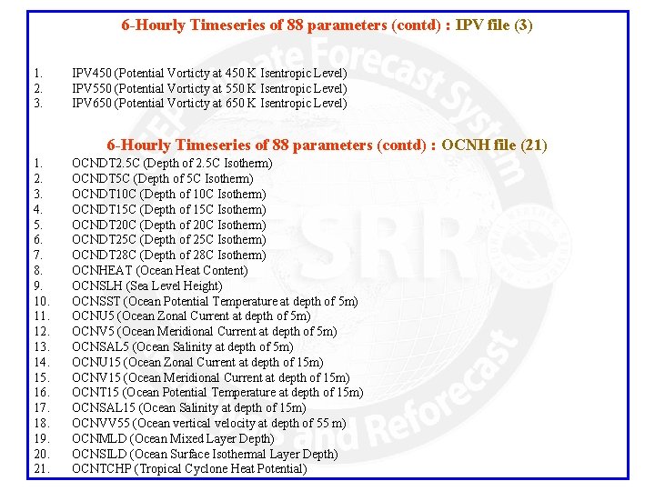
6 -Hourly Timeseries of 88 parameters (contd) : IPV file (3) 1. 2. 3. IPV 450 (Potential Vorticty at 450 K Isentropic Level) IPV 550 (Potential Vorticty at 550 K Isentropic Level) IPV 650 (Potential Vorticty at 650 K Isentropic Level) 6 -Hourly Timeseries of 88 parameters (contd) : OCNH file (21) 1. 2. 3. 4. 5. 6. 7. 8. 9. 10. 11. 12. 13. 14. 15. 16. 17. 18. 19. 20. 21. OCNDT 2. 5 C (Depth of 2. 5 C Isotherm) OCNDT 5 C (Depth of 5 C Isotherm) OCNDT 10 C (Depth of 10 C Isotherm) OCNDT 15 C (Depth of 15 C Isotherm) OCNDT 20 C (Depth of 20 C Isotherm) OCNDT 25 C (Depth of 25 C Isotherm) OCNDT 28 C (Depth of 28 C Isotherm) OCNHEAT (Ocean Heat Content) OCNSLH (Sea Level Height) OCNSST (Ocean Potential Temperature at depth of 5 m) OCNU 5 (Ocean Zonal Current at depth of 5 m) OCNV 5 (Ocean Meridional Current at depth of 5 m) OCNSAL 5 (Ocean Salinity at depth of 5 m) OCNU 15 (Ocean Zonal Current at depth of 15 m) OCNV 15 (Ocean Meridional Current at depth of 15 m) OCNT 15 (Ocean Potential Temperature at depth of 15 m) OCNSAL 15 (Ocean Salinity at depth of 15 m) OCNVV 55 (Ocean vertical velocity at depth of 55 m) OCNMLD (Ocean Mixed Layer Depth) OCNSILD (Ocean Surface Isothermal Layer Depth) OCNTCHP (Tropical Cyclone Heat Potential)

THANK YOU CFSR Website : http: //cfs. ncep. noaa. gov/cfsr Email : cfs@noaa. gov