NCEP Climate Forecast Systems T 62 vs T

 – T 62 1. 2. 3. Atmospheric component • •")


 and")
 and")


 NINO 4 TAUX NINO 3. 4 SST")
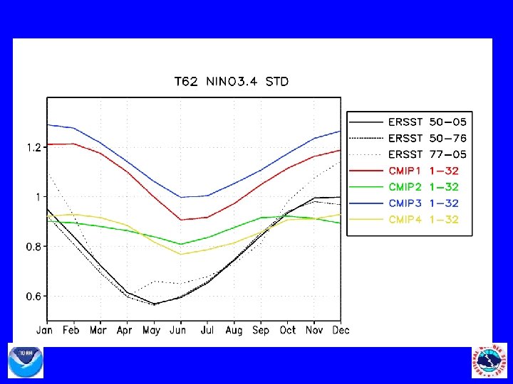
 is strongest during Feb-Mar")

 is strongest during Nov-Jan and weakest")


- Slides: 49
NCEP Climate Forecast Systems T 62 vs. T 126: Annual Cycle, ENSO and its Decadal Changes Yan Xue Climate Prediction Center Acknowledgements: Suru Saha, Wanqui Wang, Kyong-Hwan Seo, Boyin Huang
Climate Forecast System (CFS) – T 62 1. 2. 3. Atmospheric component • • Global Forecast System 2003 T 62 in horizontal; 64 layers in vertical Oceanic component • • • GFDL MOM 3 1/3°´ 1° in tropics; 1°´ 1° in extratropics; 40 layers Quasi-global domain (74°S to 64°N) Coupled model • • • Once-a-day coupling No flux correction Sea ice extent taken as observed climatology
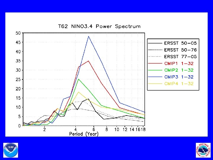
Wang et al. 2005 • • • Climatology well simulated NINO 3. 4 amplitude larger than observation Phase-locking to end of year Early onset and late decay ENSO too regular Kirtman 2005 • • Model’s low frequency modes differ from observation Initialization shock
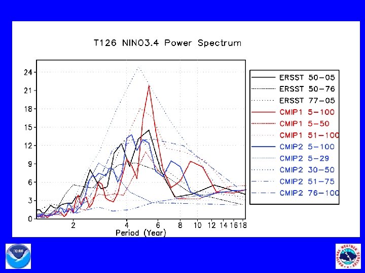
T 62 vs. T 126 • Climate Forecast System T 62 went operational in 2004. • Keeping the oceanic component unchanged, the horizontal resolution of the atmospheric component was increased from T 62 to T 126. • Two sets of simulations with T 126, each 100 year long, were studied here. • Four sets of simulations with T 62, each 32 year long, were studied here.
S W W S
Penland Saha, 2005 T 62 T 126 OBS
Motivation • Characteristics of observed ENSO change with time: pre- and post 1976 • Mechanisms for decadal modulations of ENSO: – Background state changes (Fedorov and Philander 2000) – Interaction between annual cycle and ENSO – Atmospheric noise forcings – Interactions between the tropics and subtropics – Nonlinear dynamics • What are the mechanisms controlling ENSO characteristics in T 62 and T 126? • What are the biases of the mean and annual cycle in T 62 and T 126? • How do the biases in models influence their ENSO characteristics? • Why do the ENSO characteristics in T 126 change from decade to decade?
Data • ERSST in 1950 -2005 • FSU wind stress in 1978 -2005 • CMAP precipitation in 1979 -2003 • Depth of 20 o. C isotherm from NCEP’s Global Ocean Data Assimilation System in 1979 -2005 • Monthly and daily fields from T 62 • Monthly and daily fields from T 126 Methodology • Spectrum analysis • Linear regression • Composite analysis • Interannual Coupling Strength and Thermocline Coupling Strength • Intraseasonal variance in 20 -90 days
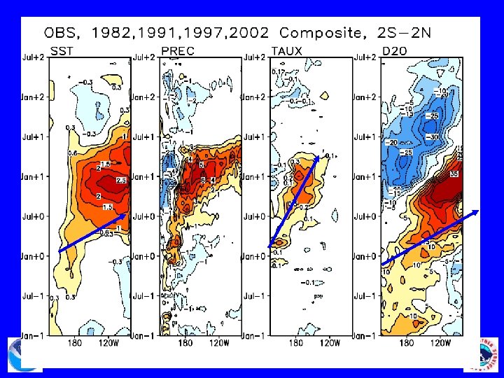
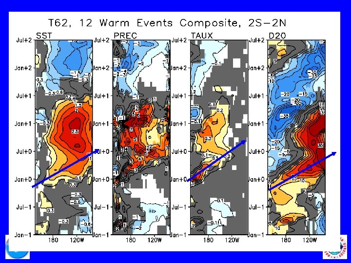
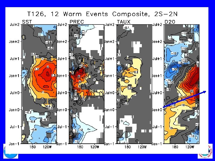
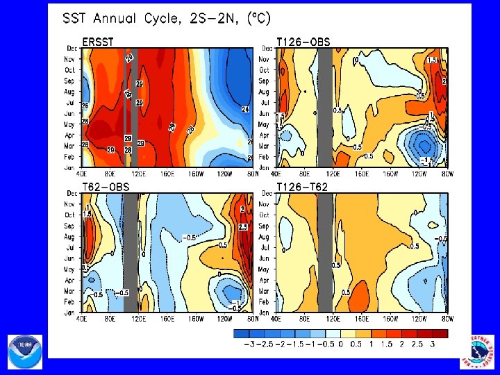
• Amplitude of SST anom. in T 62 and T 126 (1. 2 o. C) is similar to obs except the maximum center is detached from the coast. • Spatial structure of SST anom. is similar to obs except its meridional width is a little too narrow.
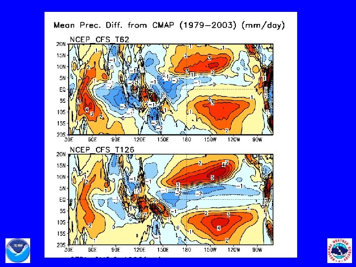
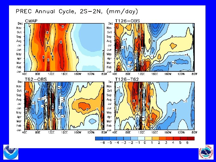
• Amplitude of prec. anom. in T 62 and T 126 (2. 5 mm/day) is similar to obs except there are two maximum centers located to north and south of the equator. • Spatial structure of prec. anom. is similar to obs except convection south of equator extended too far eastward, subsidence over Indonesian continent is too weak and subsidence to north of ITCZ too strong.
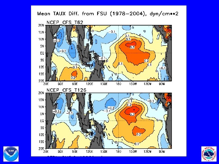
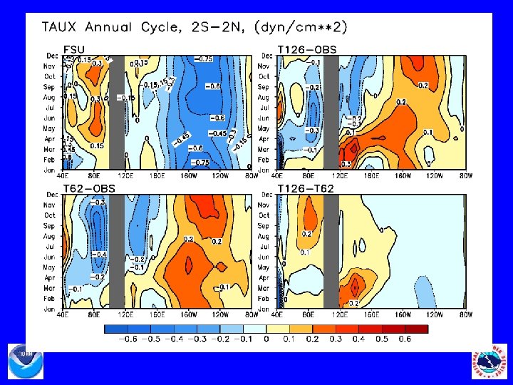
• Amplitude of westerly anom. in T 62 (1. 2 dyn/cm 2) and T 126 (0. 9 dyn/cm 2) is smaller than that of obs (1. 5 dyn/cm 2), but easterly anom. to north of westerly center is too strong. • Spatial structure of zonal wind stress anom. is similar to that of obs except its meridional width is too narrow.
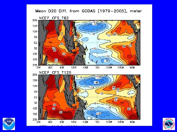
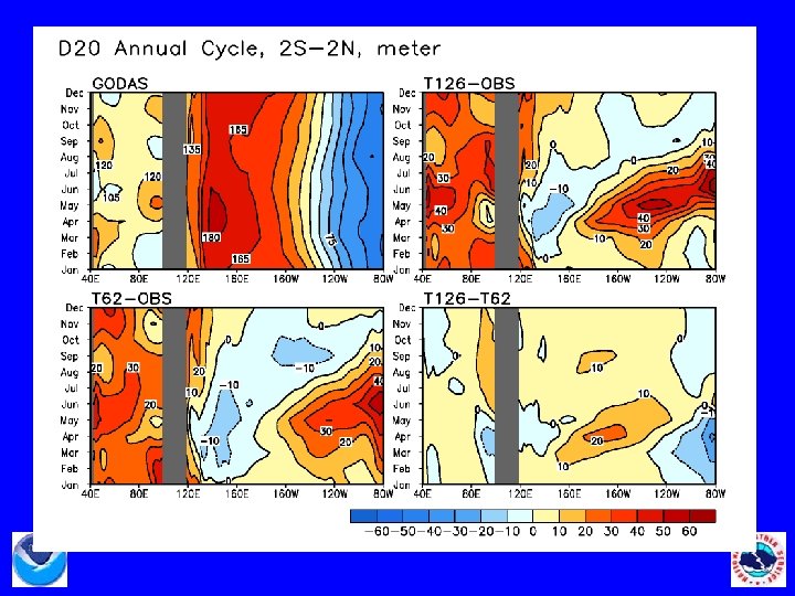
• Amplitude of positive D 20 anom. in T 62 (20 meter) and T 126 (20 meter) is a little larger than that of obs (15 meter). • Positive center in the eastern Pacific is too equatorially confined, and the negative center in the north-western Pacific is located too close to the equator, and extended too far eastward.
Lag • SST anom. in T 62 propagates eastward, while SST anom. in T 126 is largely stationary, close to obs. . • Duration of SST anom. in T 62 and T 126 are too long compared to obs. . • Onset of ENSO is too early in T 62.
Lag • Prec. anom. in T 62 propagates from the western Pacific to eastern Pacific, close to obs. , while prec. anom. in T 126 has no propagation. • Prec. anom. in the far western Pacific in T 62 and T 126 is too weak. • Prec. anom. in T 62 is too large in the Indian Ocean.
Lag • Zonal wind stress anom. in T 62 propagates from the western Pacific to central Pacific, similar to obs. , while T 126 anom. is largely stationary. • Easterly anom. in the far western Pacific in T 126 is too weak. • Anom. in the Indian Ocean in T 62 is too strong.
Lag • D 20 anom. in T 62 propagates from the western Pacific to eastern Pacific, similar to obs. , while T 126 anom. propagates little. • T 62 has too strong D 20 precursor. • T 62 has too strong amplitude in the Indian Ocean.
late onset 4 warm events early onset: > 0. 5 o. C Yr 0 normal onset (4): Mar+0 – May+0 late onset (1): Aug 2 year peaks 12 warm events normal onset (12): early onset Dec-1 – Apr+0 late onset (3): Jul+0 – Sep+0 late onset early onset (4): Sep-1 – Nov-1 early onset
12 warm events early onset: > 0. 5 o. C Yr 0 normal onset (12): Jan+0 (3), Apr +0 (1), May+0 (1), Jun+0 (3), Jul+0 (2), Aug+0 (2) early onset (2): Oct-1
Air-See Feedback Loop Interannual Coupling Strength (ICS) NINO 4 TAUX NINO 3. 4 SST NINO 3 SST Thermocline Coupling Strength (TCS) D 20
warm SST large SST gradient • Interannual Coupling Strength (ICS) is strongest during Feb-Mar and Aug -Sep, and weakest during May-Jul and Nov-Dec. • ICS of T 62 is weaker than that of observation.
OBS T 62 T 126 CMIP 1 T 126 CMIP 2 • Both T 62 and T 126 are more stable than that of observation. • T 62 is more unstable than T 126 during Nov-Feb.
TCS weak upwelling • Thermocline Coupling Strength (TCS) is strongest during Nov-Jan and weakest during Mar-Apr when upwelling is weakest. • TCS of T 62 is much stronger than that of observation, particularly in Feb. Apr and Jul-Sep.
TCS T 62 T 126 CMIP 1 • TCS of T 62 and T 126 are both stronger than that of observation, particularly in Feb-Apr and Jul-Sep. • T 62 is more unstable than T 126 in May-Sep.
OBS T 62 T 126 CMIP 1 T 126 CMIP 2 • Both T 62 and T 126 are more stable than that of observation. • T 62 is more unstable than T 126 during Nov-Feb.
T 126 CMIP 1 51 -100 yr T 62 CMIP 1 T 126 CMIP 1 1 -50 yr T 62 CMIP 1 T 126 CMIP 1 51 -100
T 126 CMIP 2
S 1 W 1 S 1 W 2 S 2
CMIP 1 S 1 – W 1
CMIP 2 S 1 – W 1
CMIP 2 W 2 – S 1
CMIP 2 S 2 – W 2
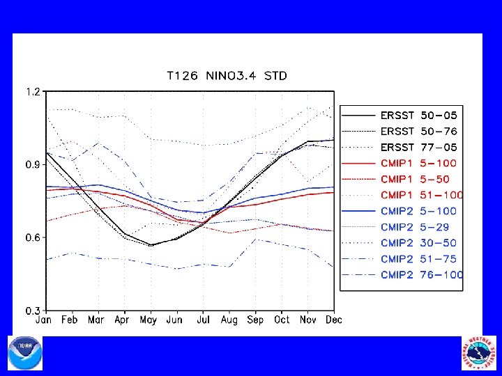
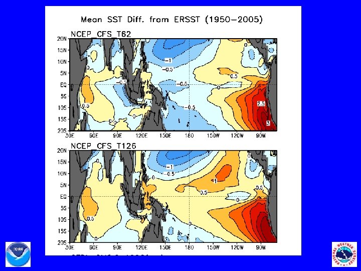
Summary • T 62 and T 126 have similar mean biases – Negative SST biases (-1 o. C) in north-western Pacific, positive biases (2 o. C) in south-eastern Pacific – Double ITCZ and too little prec. in the equatorial western Pacific • T 62 and T 126 have different biases in annual cycle on the equator – SST in the eastern Pacific peaks in May in T 62 and in June in T 126 – T 126 has eastward propagating westerly and rain band in early spring in the far western Pacific – Both T 62 and T 126 have too deep thermocline in June due to excessive westerly in the far western Pacific in spring • T 62 and T 126 have similar phase-locking of warm events to end of year but T 62 has onsets in Dec-1 – Apr+0 and T 126 has onsets in Jan+0 – Aug+0.
Summary • Interannual Coupling Strength of T 62 and T 126 are both weaker than that of observation, but they are compensated by their stronger Thermocline Coupling Strength. • Interannual Coupling Strength of T 126 is weaker than that of T 62 in Nov-Feb, probably due to its confined rain band to the far western Pacific and delayed eastern Pacific warming. • T 126 is more stable than T 62, and its onset of ENSO is more irregular than that of T 62, suggesting that the system is near neutral and atmospheric stochastic forcings could play significant roles on its ENSO evolution. • Decadal modulations of ENSO are related to background state changes – cool in the western Pacific, warm in the eastern Pacific, westerly anom. near the dateline, deep thermocline in the eastern Pacific and shallow thermocline in the western Pacific favor strong ENSO variability.
Future Work • Explore the impacts of atmospheric noise forcings on ENSO. • Explain why T 62 has a much earlier onset than T 126 does. • Explore the roles of the Indian Ocean. • Explore the roles of the subtropical Rossby waves on ENSO. • Explore mechanisms for decadal modulations of ENSO.