Advanced Forecasting Copyright c 2008 by The Mc

Advanced Forecasting Copyright (c) 2008 by The Mc. Graw-Hill Companies. This material is intended solely for educational use by licensed users of Learning. Stats. It may not be copied or resold for profit.

Copyright Notice Portions of MINITAB Statistical Software input and output contained in this document are printed with permission of Minitab, Inc. MINITAB TM is a trademark of Minitab Inc. in the United States and other countries and is used herein with the owner's permission.

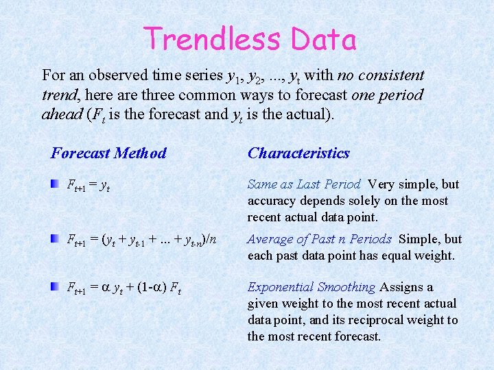
Trendless Data For an observed time series y 1, y 2, . . . , yt with no consistent trend, here are three common ways to forecast one period ahead (Ft is the forecast and yt is the actual). Forecast Method Characteristics Ft+1 = yt Same as Last Period Very simple, but accuracy depends solely on the most recent actual data point. Ft+1 = (yt + yt-1 +. . . + yt-n)/n Average of Past n Periods Simple, but each past data point has equal weight. Ft+1 = a yt + (1 -a) Ft Exponential Smoothing Assigns a given weight to the most recent actual data point, and its reciprocal weight to the most recent forecast.

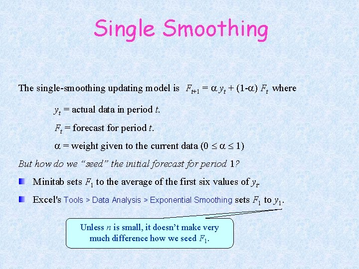
Single Smoothing The single-smoothing updating model is Ft+1 = a yt + (1 -a) Ft where yt = actual data in period t. Ft = forecast for period t. a = weight given to the current data (0 a 1) But how do we “seed” the initial forecast for period 1? Minitab sets F 1 to the average of the first six values of yt. Excel's Tools > Data Analysis > Exponential Smoothing sets F 1 to y 1. Unless n is small, it doesn’t make very much difference how we seed F 1.

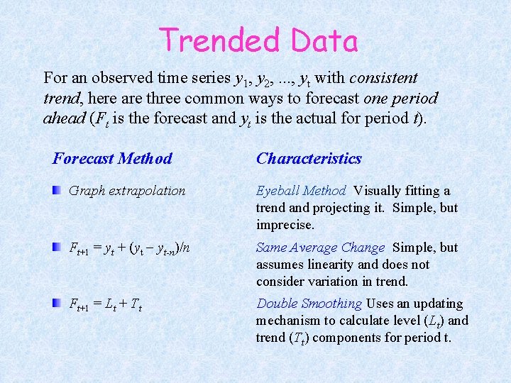
Trended Data For an observed time series y 1, y 2, . . . , yt with consistent trend, here are three common ways to forecast one period ahead (Ft is the forecast and yt is the actual for period t). Forecast Method Characteristics Graph extrapolation Eyeball Method Visually fitting a trend and projecting it. Simple, but imprecise. Ft+1 = yt + (yt yt-n)/n Same Average Change Simple, but assumes linearity and does not consider variation in trend. Ft+1 = Lt + Tt Double Smoothing Uses an updating mechanism to calculate level (Lt) and trend (Tt) components for period t.

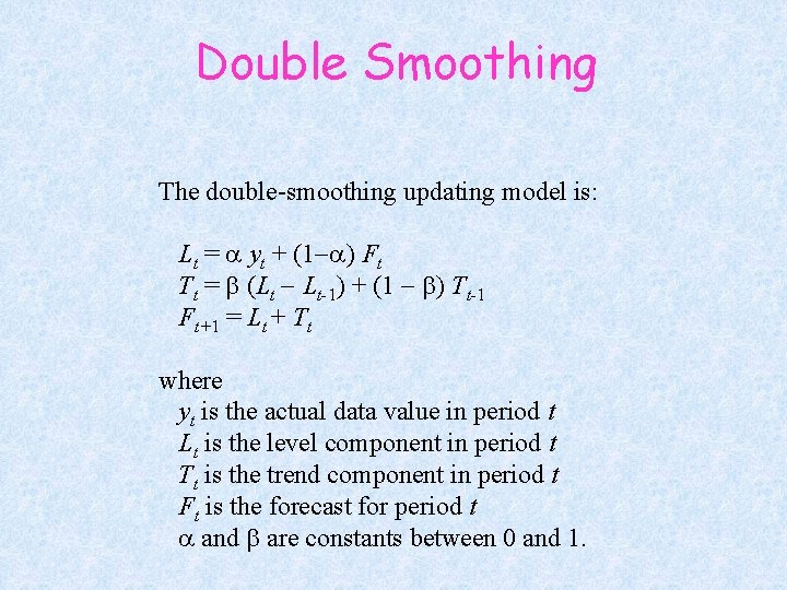
Double Smoothing The double-smoothing updating model is: Lt = a yt + (1 a) Ft Tt = b (Lt Lt-1) + (1 b) Tt-1 Ft+1 = Lt + Tt where yt is the actual data value in period t Lt is the level component in period t Tt is the trend component in period t Ft is the forecast for period t a and b are constants between 0 and 1.

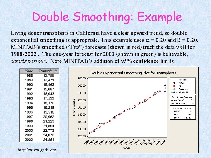
Double Smoothing: Example Living donor transplants in California have a clear upward trend, so double exponential smoothing is appropriate. This example uses a = 0. 20 and b = 0. 20. MINITAB’s smoothed (“Fits”) forecasts (shown in red) track the data well for 1988 -2002. The one-year forecast for 2003 (shown in green) is believable, ceteris paribus. Note MINITAB’s addition of 95% confidence limits. http: //www. gsds. org

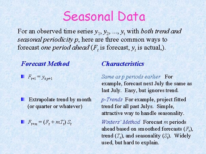
Seasonal Data For an observed time series y 1, y 2, . . . , yt with both trend and seasonal periodicity p, here are three common ways to forecast one period ahead (Ft is forecast, yt is actual, ). Forecast Method Characteristics Ft+1 = yt-p+1 Same as p periods earlier For example, forecast next July the same as last July. Easy, but ignores trend. Extrapolate trend by month (or quarter or whatever) p-Trends For example, project fitted trend for all past Julys. Simple, attractive way to handle seasonality. Ft+m = (Ft + m. Tt) St Winters’ Method Forecast m periods ahead based on smoothed forecasts (Ft), trend (Tt), and seasonality (St). Widely used, but hard to explain.

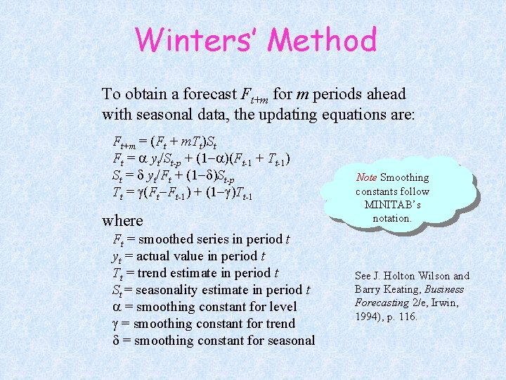
Winters’ Method To obtain a forecast Ft+m for m periods ahead with seasonal data, the updating equations are: Ft+m = (Ft + m. Tt)St Ft = a yt/St-p + (1 a)(Ft-1 + Tt-1) St = d yt/Ft + (1 d)St-p Tt = g(Ft Ft-1) + (1 g)Tt-1 where Ft = smoothed series in period t yt = actual value in period t Tt = trend estimate in period t St = seasonality estimate in period t a = smoothing constant for level g = smoothing constant for trend d = smoothing constant for seasonal Note Smoothing constants follow MINITAB’s notation. See J. Holton Wilson and Barry Keating, Business Forecasting 2/e, Irwin, 1994), p. 116.

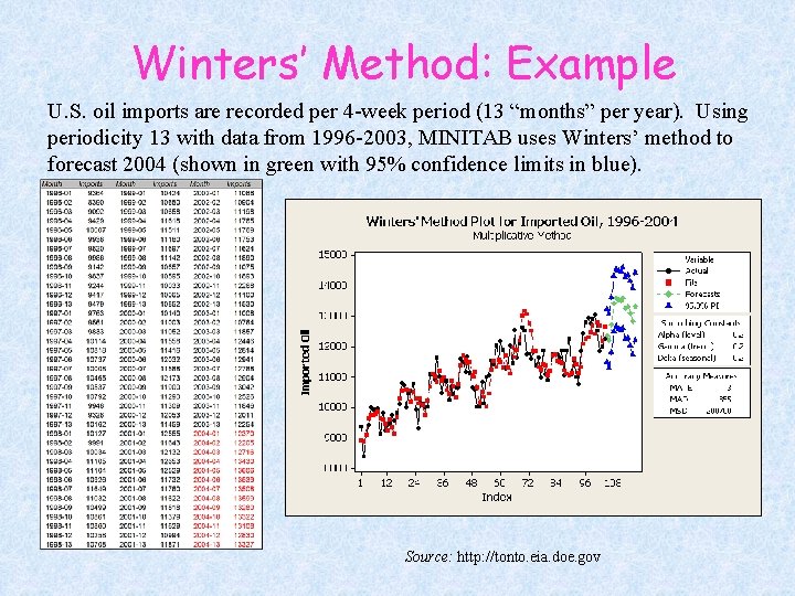
Winters’ Method: Example U. S. oil imports are recorded per 4 -week period (13 “months” per year). Using periodicity 13 with data from 1996 -2003, MINITAB uses Winters’ method to forecast 2004 (shown in green with 95% confidence limits in blue). Source: http: //tonto. eia. doe. gov

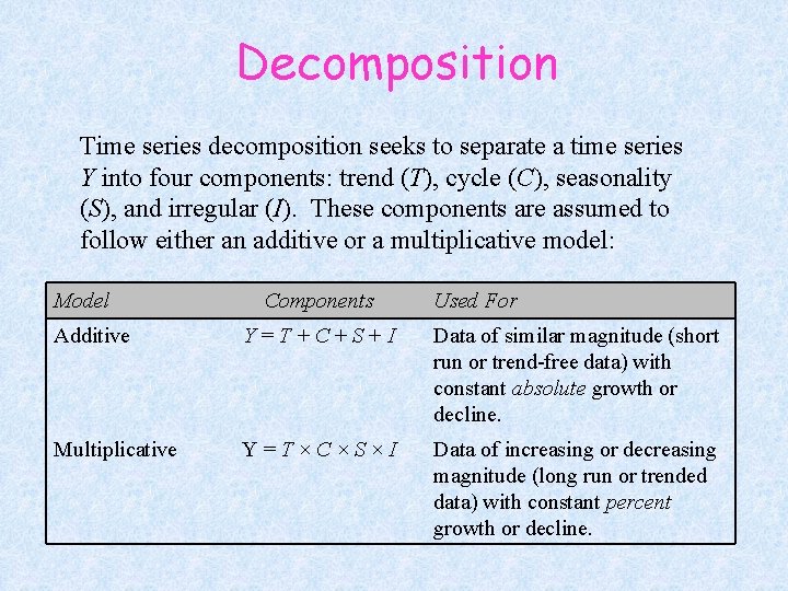
Decomposition Time series decomposition seeks to separate a time series Y into four components: trend (T), cycle (C), seasonality (S), and irregular (I). These components are assumed to follow either an additive or a multiplicative model: Model Components Used For Additive Y=T+C+S+I Data of similar magnitude (short run or trend-free data) with constant absolute growth or decline. Multiplicative Y=T×C×S×I Data of increasing or decreasing magnitude (long run or trended data) with constant percent growth or decline.

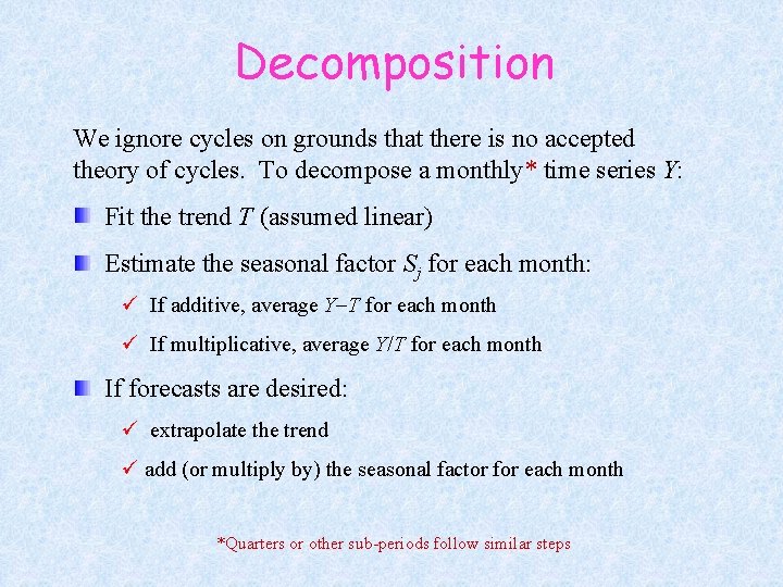
Decomposition We ignore cycles on grounds that there is no accepted theory of cycles. To decompose a monthly* time series Y: Fit the trend T (assumed linear) Estimate the seasonal factor Sj for each month: ü If additive, average Y T for each month ü If multiplicative, average Y/T for each month If forecasts are desired: ü extrapolate the trend ü add (or multiply by) the seasonal factor for each month *Quarters or other sub-periods follow similar steps

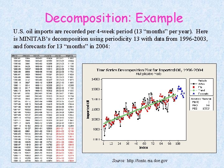
Decomposition: Example U. S. oil imports are recorded per 4 -week period (13 “months” per year). Here is MINITAB’s decomposition using periodicity 13 with data from 1996 -2003, and forecasts for 13 “months” in 2004: Source: http: //tonto. eia. doe. gov

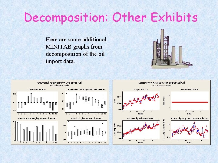
Decomposition: Other Exhibits Here are some additional MINITAB graphs from decomposition of the oil import data.

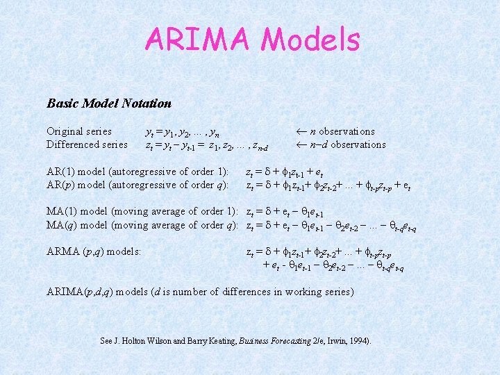
ARIMA Models Basic Model Notation Original series Differenced series yt = y 1, y 2, . . . , yn zt = yt yt-1 = z 1, z 2, . . . , zn-d AR(1) model (autoregressive of order 1): AR(p) model (autoregressive of order q): n observations n d observations zt = d + f 1 zt-1 + et zt = d + f 1 zt-1+ f 2 zt-2+. . . + ft-pzt-p + et MA(1) model (moving average of order 1): zt = d + et q 1 et-1 MA(q) model (moving average of order q): zt = d + et q 1 et-1 q 2 et-2 . . . qt-qet-q ARMA (p, q) models: zt = d + f 1 zt-1+ f 2 zt-2+. . . + ft-pzt-p + et - q 1 et-1 q 2 et-2 . . . qt-qet-q ARIMA(p, d, q) models (d is number of differences in working series) See J. Holton Wilson and Barry Keating, Business Forecasting 2/e, Irwin, 1994).

ARIMA Model identification depends on the data. It is rarely necessary to go beyond AR(1) or MA(1), although seasonal data will require fancier models. Criteria for model adequacy can be found in any forecasting textbook. Time series modeling using ARIMA is an advanced topic that requires additional study*. * See J. Holton Wilson and Barry Keating, Business Forecasting 2/e, Irwin, 1994).

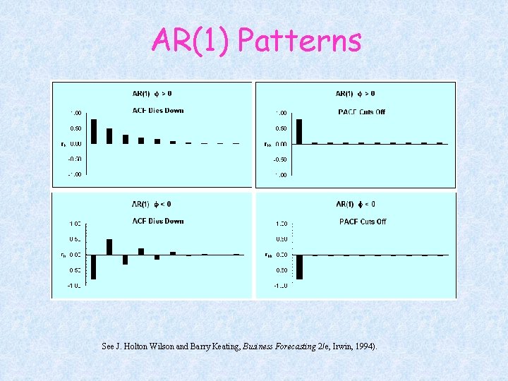
AR(1) Patterns See J. Holton Wilson and Barry Keating, Business Forecasting 2/e, Irwin, 1994).

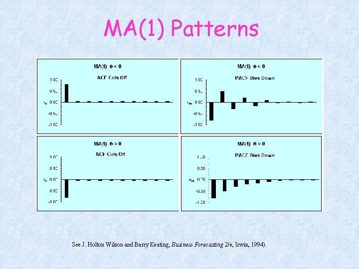
MA(1) Patterns See J. Holton Wilson and Barry Keating, Business Forecasting 2/e, Irwin, 1994).

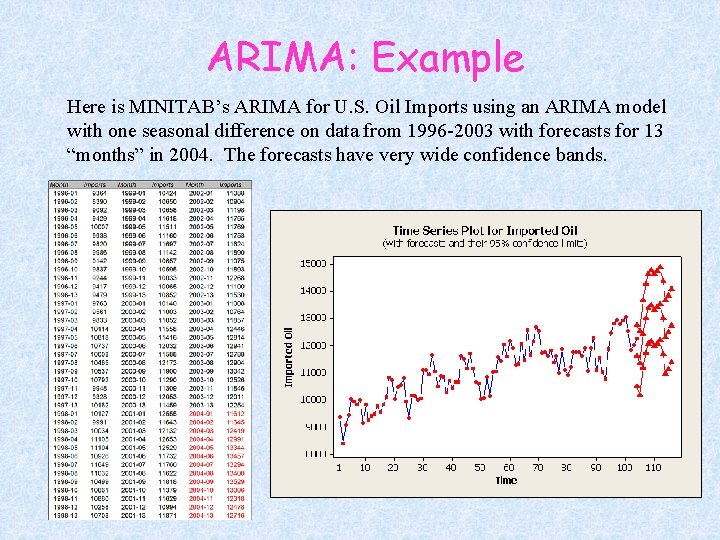
ARIMA: Example Here is MINITAB’s ARIMA for U. S. Oil Imports using an ARIMA model with one seasonal difference on data from 1996 -2003 with forecasts for 13 “months” in 2004. The forecasts have very wide confidence bands.

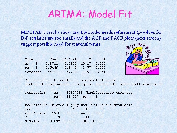
ARIMA: Model Fit MINITAB’s results show that the model needs refinement (p-values for B-P statistics are too small) and the ACF and PACF plots (next screen) suggest possible need for seasonal terms. Type AR 1 MA 1 Constant Coef 0. 8722 0. 5449 54. 61 SE Coef 0. 0850 0. 1445 27. 66 T 10. 27 3. 77 1. 97 P 0. 000 0. 051 Differencing: 0 regular, 1 seasonal of order 13 Number of observations: Original series 104, after differencing 91 Residuals: SS = MS = 29397038 (backforecasts excluded) 334057 DF = 88 Modified Box-Pierce (Ljung-Box) Chi-Square statistic Lag 12 24 36 48 Chi-Square 17. 8 55. 5 66. 1 75. 5 DF 9 21 33 45 P-Value 0. 037 0. 000 0. 001 0. 003

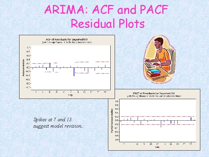
ARIMA: ACF and PACF Residual Plots Spikes at 7 and 13 suggest model revision.

Other Methods Seasonal binaries in regression Moving average to remove trend (instead of linear OLS trend) then decomposition on residuals Ad hoc methods

Final Advice Occam's Razor Given two sufficient explanations, we prefer the simpler. Named for the English philosopher William of Occam (d. 1349). Remember Occam’s Razor Don’t be dazzled by equations Think about underlying causes Are your forecasts credible? Clean, simple graphs help