TIME SERIES MODELS MOVING AVERAGES Definitions Forecast is

TIME SERIES MODELS – MOVING AVERAGES

Definitions • Forecast is a prediction of future events used for planning process. • Time Series is the repeated observations of demand for a service or product in their order of occurrence (sequence of time).

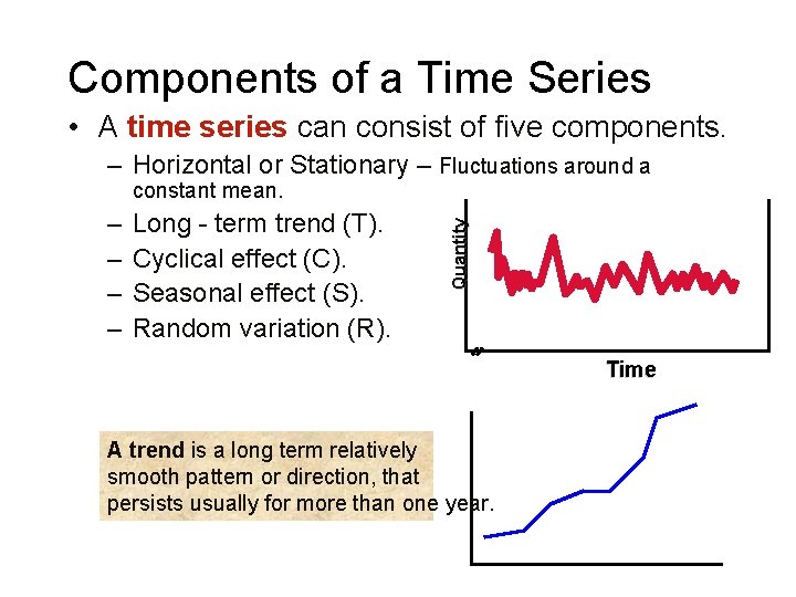
Components of a Time Series • A time series can consist of five components. – Horizontal or Stationary – Fluctuations around a – – Long - term trend (T). Cyclical effect (C). Seasonal effect (S). Random variation (R). Quantity constant mean. Time A trend is a long term relatively smooth pattern or direction, that persists usually for more than one year.

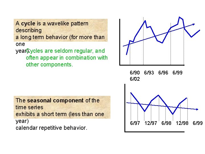
A cycle is a wavelike pattern describing a long term behavior (for more than one year). Cycles are seldom regular, and often appear in combination with other components. 6/90 6/93 6/96 6/99 6/02 The seasonal component of the time series exhibits a short term (less than one year) calendar repetitive behavior. 6/97 12/97 6/98 12/98 6/99

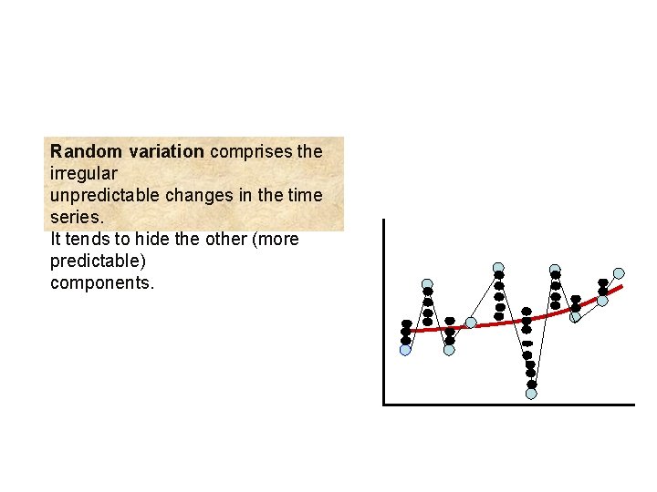
Random variation comprises the irregular unpredictable changes in the time series. It tends to hide the other (more predictable) components.

Time Series Forecasting Methods • Consider models applicable to time series data with seasonal, trend, or both seasonal and trend component and stationary data.

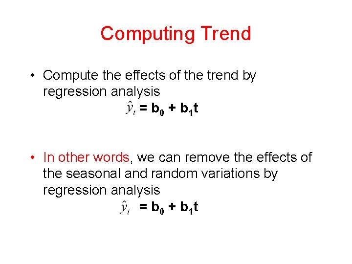
Computing Trend • Compute the effects of the trend by regression analysis = b 0 + b 1 t • In other words, we can remove the effects of the seasonal and random variations by regression analysis = b 0 + b 1 t

Moving Average and Exponential Smoothing Methods • Consider models applicable to time series data for extracting seasonal component. Forecasting methods discussed can be classified as: • – Averaging methods. • – Equally weighted observations Exponential Smoothing methods. • • • Unequal set of weights to past data, where the weights decay exponentially from the most recent to the most distant data points. All methods in this group require that certain parameters to be defined. These parameters (with values between 0 and 1) will determine the unequal weights to be applied to past data.

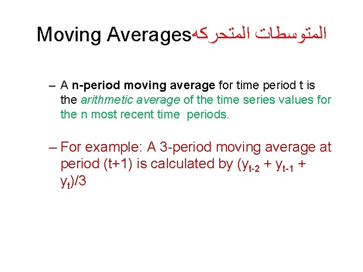
Moving Averages ﺍﻟﻤﺘﻮﺳﻄﺎﺕ ﺍﻟﻤﺘﺤﺮﻛﻪ – A n-period moving average for time period t is the arithmetic average of the time series values for the n most recent time periods. – For example: A 3 -period moving average at period (t+1) is calculated by (yt-2 + yt-1 + yt)/3

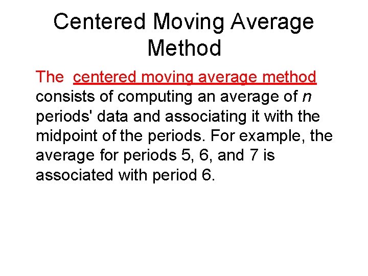
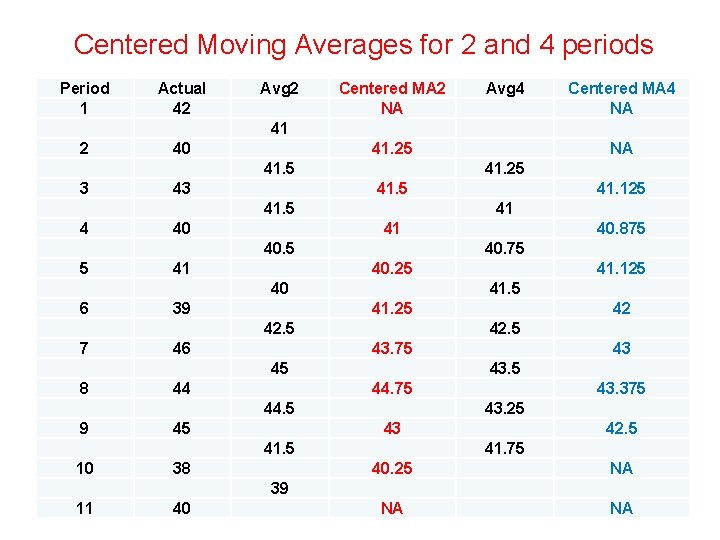
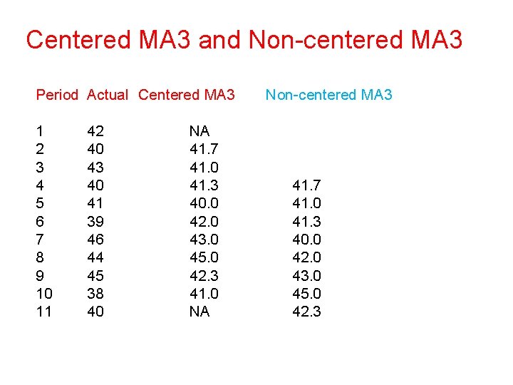
Centered Moving Average Method The centered moving average method consists of computing an average of n periods' data and associating it with the midpoint of the periods. For example, the average for periods 5, 6, and 7 is associated with period 6.

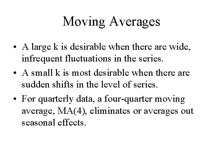
Moving Averages • A large k is desirable when there are wide, infrequent fluctuations in the series. • A small k is most desirable when there are sudden shifts in the level of series. • For quarterly data, a four-quarter moving average, MA(4), eliminates or averages out seasonal effects.

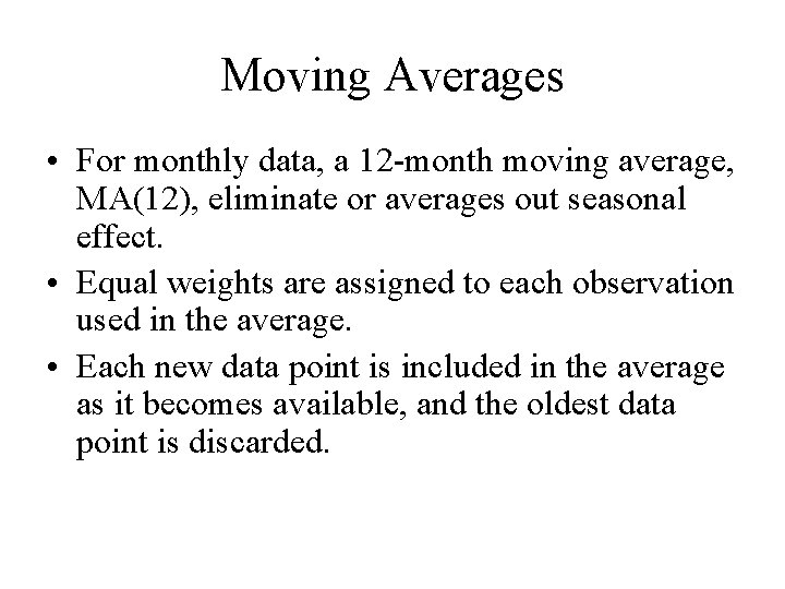
Moving Averages • For monthly data, a 12 -month moving average, MA(12), eliminate or averages out seasonal effect. • Equal weights are assigned to each observation used in the average. • Each new data point is included in the average as it becomes available, and the oldest data point is discarded.

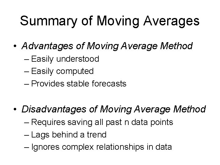
Summary of Moving Averages • Advantages of Moving Average Method – Easily understood – Easily computed – Provides stable forecasts • Disadvantages of Moving Average Method – Requires saving all past n data points – Lags behind a trend – Ignores complex relationships in data

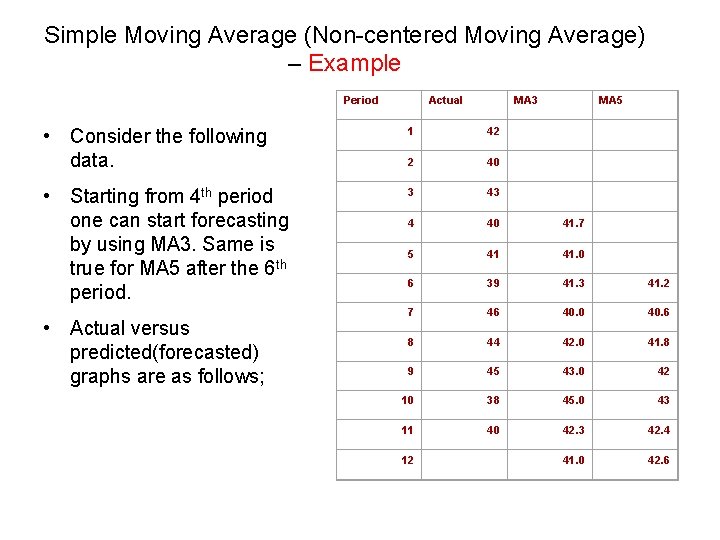
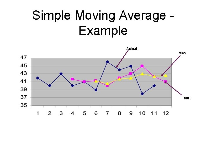
Simple Moving Average (Non-centered Moving Average) – Example Period Actual MA 3 MA 5 • Consider the following data. 1 42 2 40 • Starting from 4 th period one can start forecasting by using MA 3. Same is true for MA 5 after the 6 th period. 3 43 4 40 41. 7 5 41 41. 0 6 39 41. 3 41. 2 7 46 40. 0 40. 6 8 44 42. 0 41. 8 9 45 43. 0 42 10 38 45. 0 43 11 40 42. 3 42. 4 41. 0 42. 6 • Actual versus predicted(forecasted) graphs are as follows; 12

Simple Moving Average Example Actual MA 5 MA 3

Centered Moving Averages for 2 and 4 periods Period 1 Actual 42 Avg 2 Centered MA 2 NA Avg 4 Centered MA 4 NA 41 2 40 41. 25 41. 5 3 43 41. 25 41. 5 4 40 41 41 40. 25 39 41. 25 46 43. 75 44 44. 75 45 43. 375 43. 25 43 41. 5 10 43 43. 5 44. 5 9 42 42. 5 45 8 41. 125 41. 5 42. 5 7 40. 875 40 6 41. 125 41 40. 5 5 NA 38 42. 5 41. 75 40. 25 NA NA NA 39 11 40

Centered MA 3 and Non-centered MA 3 Period Actual Centered MA 3 1 2 3 4 5 6 7 8 9 10 11 42 40 43 40 41 39 46 44 45 38 40 NA 41. 7 41. 0 41. 3 40. 0 42. 0 43. 0 45. 0 42. 3 41. 0 NA Non-centered MA 3 41. 7 41. 0 41. 3 40. 0 42. 0 43. 0 45. 0 42. 3