Analysis of Algorithms Input Algorithm Output An algorithm

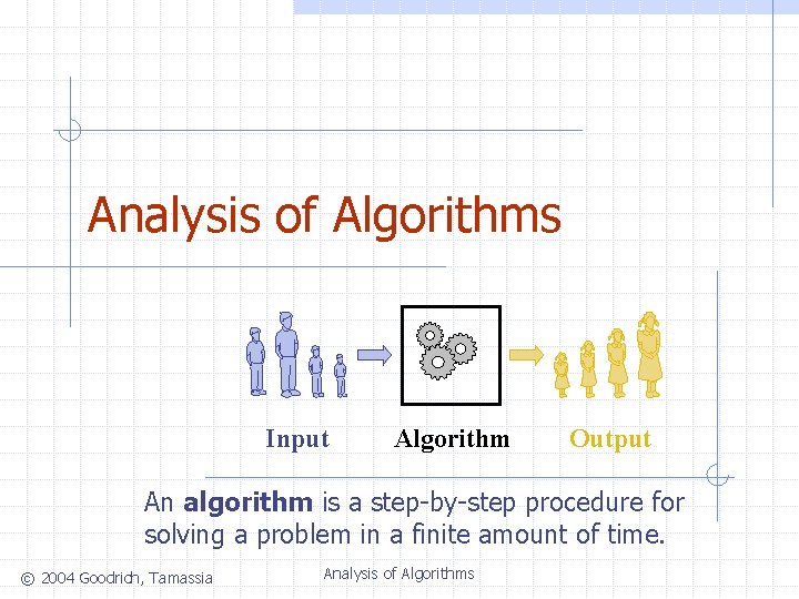
Analysis of Algorithms Input Algorithm Output An algorithm is a step-by-step procedure for solving a problem in a finite amount of time. © 2004 Goodrich, Tamassia Analysis of Algorithms

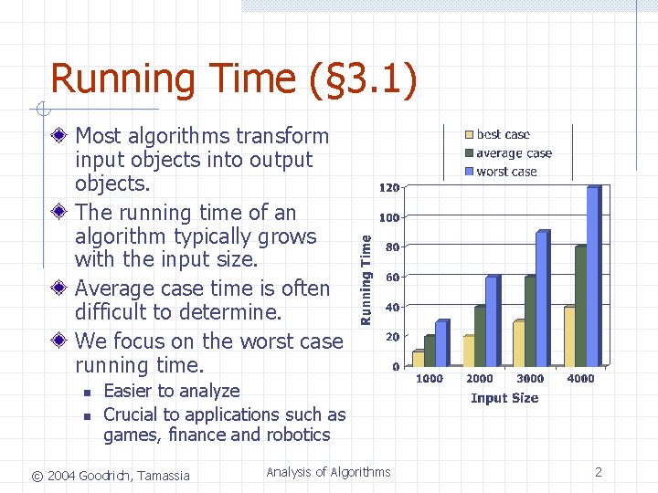
Running Time (§ 3. 1) Most algorithms transform input objects into output objects. The running time of an algorithm typically grows with the input size. Average case time is often difficult to determine. We focus on the worst case running time. n n Easier to analyze Crucial to applications such as games, finance and robotics © 2004 Goodrich, Tamassia Analysis of Algorithms 2

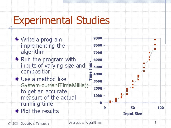
Experimental Studies Write a program implementing the algorithm Run the program with inputs of varying size and composition Use a method like System. current. Time. Millis() to get an accurate measure of the actual running time Plot the results © 2004 Goodrich, Tamassia Analysis of Algorithms 3

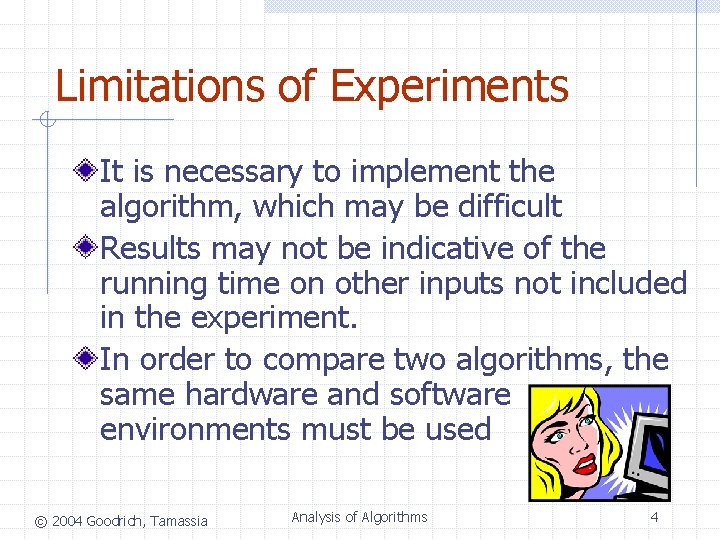
Limitations of Experiments It is necessary to implement the algorithm, which may be difficult Results may not be indicative of the running time on other inputs not included in the experiment. In order to compare two algorithms, the same hardware and software environments must be used © 2004 Goodrich, Tamassia Analysis of Algorithms 4

Theoretical Analysis Uses a high-level description of the algorithm instead of an implementation Characterizes running time as a function of the input size, n. Takes into account all possible inputs Allows us to evaluate the speed of an algorithm independent of the hardware/software environment © 2004 Goodrich, Tamassia Analysis of Algorithms 5

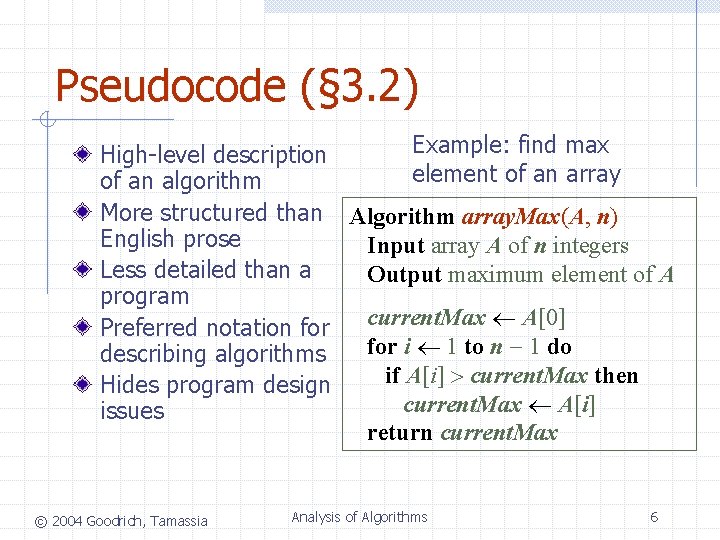
Pseudocode (§ 3. 2) Example: find max High-level description element of an array of an algorithm More structured than Algorithm array. Max(A, n) English prose Input array A of n integers Less detailed than a Output maximum element of A program current. Max A[0] Preferred notation for i 1 to n 1 do describing algorithms if A[i] current. Max then Hides program design current. Max A[i] issues return current. Max © 2004 Goodrich, Tamassia Analysis of Algorithms 6

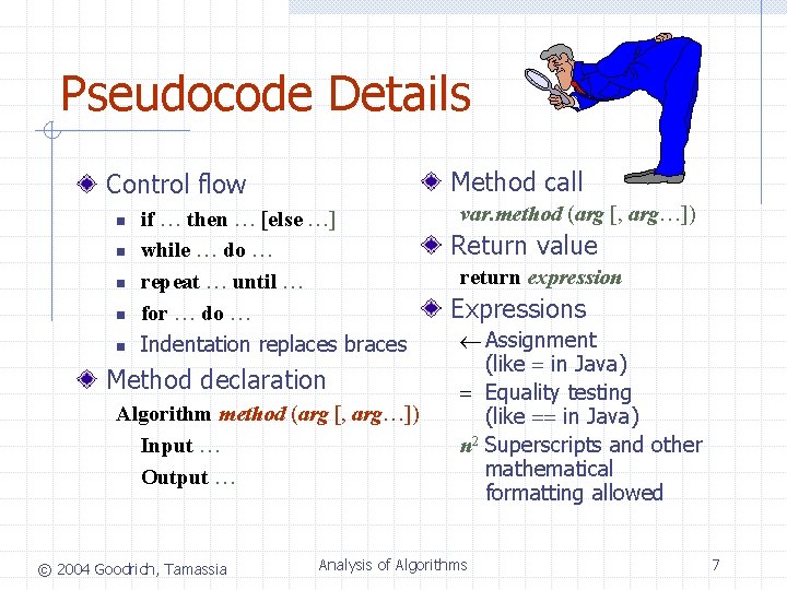
Pseudocode Details Method call Control flow n n n if … then … [else …] while … do … repeat … until … for … do … Indentation replaces braces Method declaration Algorithm method (arg [, arg…]) Input … Output … © 2004 Goodrich, Tamassia var. method (arg [, arg…]) Return value return expression Expressions Assignment (like in Java) Equality testing (like in Java) n 2 Superscripts and other mathematical formatting allowed Analysis of Algorithms 7

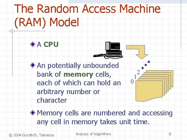
The Random Access Machine (RAM) Model A CPU An potentially unbounded bank of memory cells, each of which can hold an arbitrary number or character 0 2 1 Memory cells are numbered and accessing any cell in memory takes unit time. © 2004 Goodrich, Tamassia Analysis of Algorithms 8

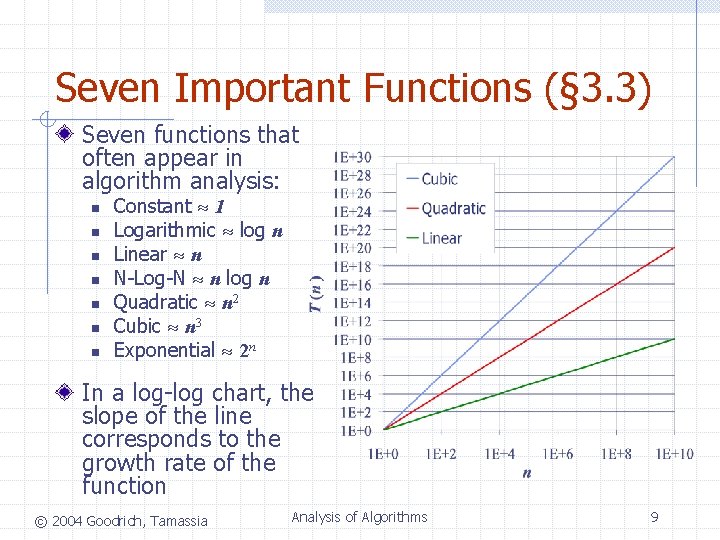
Seven Important Functions (§ 3. 3) Seven functions that often appear in algorithm analysis: n n n n Constant 1 Logarithmic log n Linear n N-Log-N n log n Quadratic n 2 Cubic n 3 Exponential 2 n In a log-log chart, the slope of the line corresponds to the growth rate of the function © 2004 Goodrich, Tamassia Analysis of Algorithms 9

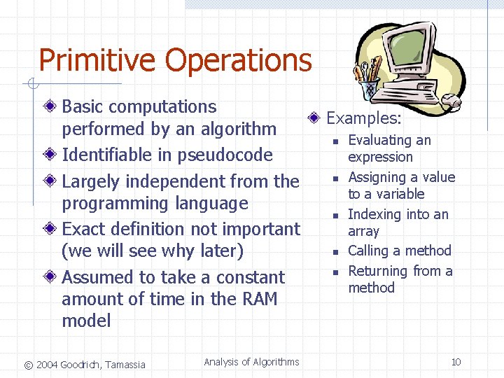
Primitive Operations Basic computations performed by an algorithm Identifiable in pseudocode Largely independent from the programming language Exact definition not important (we will see why later) Assumed to take a constant amount of time in the RAM model © 2004 Goodrich, Tamassia Analysis of Algorithms Examples: n n n Evaluating an expression Assigning a value to a variable Indexing into an array Calling a method Returning from a method 10

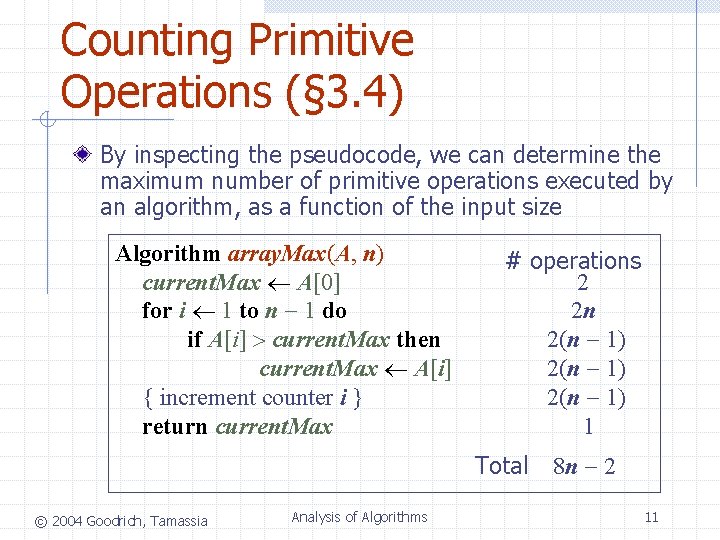
Counting Primitive Operations (§ 3. 4) By inspecting the pseudocode, we can determine the maximum number of primitive operations executed by an algorithm, as a function of the input size Algorithm array. Max(A, n) current. Max A[0] for i 1 to n 1 do if A[i] current. Max then current. Max A[i] { increment counter i } return current. Max # operations 2 2 n 2(n 1) 1 Total © 2004 Goodrich, Tamassia Analysis of Algorithms 8 n 2 11

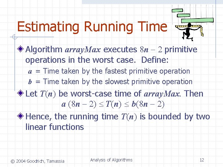
Estimating Running Time Algorithm array. Max executes 8 n 2 primitive operations in the worst case. Define: a = Time taken by the fastest primitive operation b = Time taken by the slowest primitive operation Let T(n) be worst-case time of array. Max. Then a (8 n 2) T(n) b(8 n 2) Hence, the running time T(n) is bounded by two linear functions © 2004 Goodrich, Tamassia Analysis of Algorithms 12

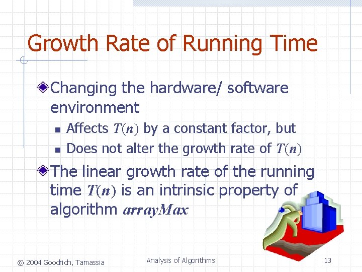
Growth Rate of Running Time Changing the hardware/ software environment n n Affects T(n) by a constant factor, but Does not alter the growth rate of T(n) The linear growth rate of the running time T(n) is an intrinsic property of algorithm array. Max © 2004 Goodrich, Tamassia Analysis of Algorithms 13

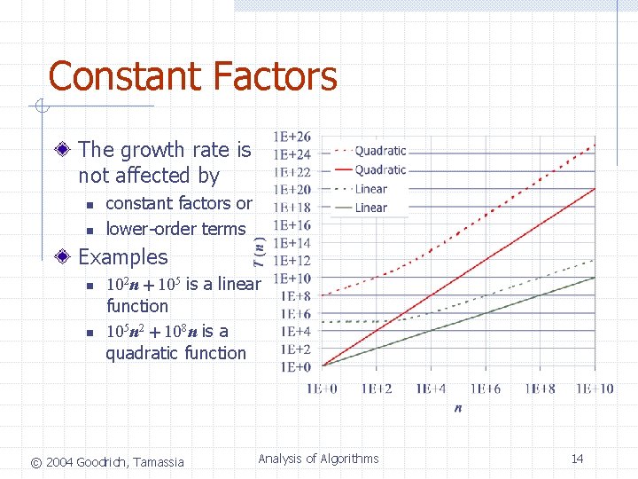
Constant Factors The growth rate is not affected by n n constant factors or lower-order terms Examples n n 102 n + 105 is a linear function 105 n 2 + 108 n is a quadratic function © 2004 Goodrich, Tamassia Analysis of Algorithms 14

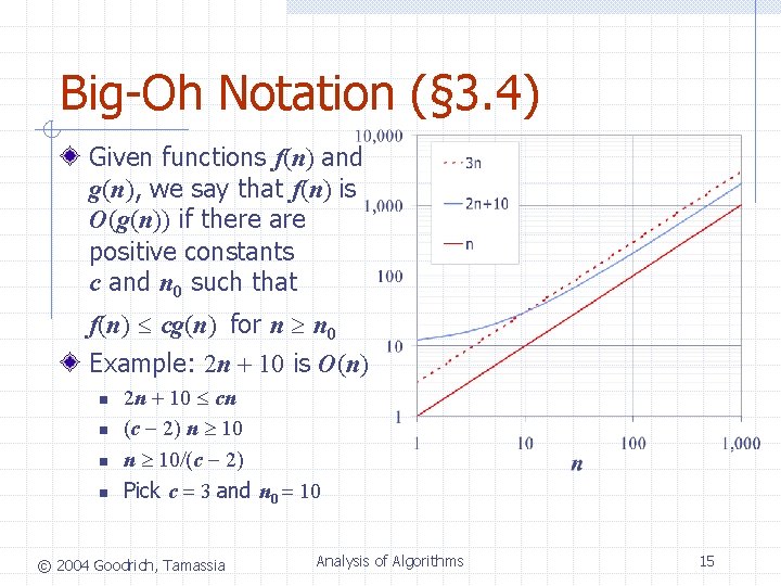
Big-Oh Notation (§ 3. 4) Given functions f(n) and g(n), we say that f(n) is O(g(n)) if there are positive constants c and n 0 such that f(n) cg(n) for n n 0 Example: 2 n + 10 is O(n) n n 2 n + 10 cn (c 2) n 10/(c 2) Pick c 3 and n 0 10 © 2004 Goodrich, Tamassia Analysis of Algorithms 15

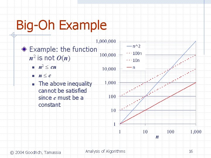
Big-Oh Example: the function n 2 is not O(n) n n 2 cn n c The above inequality cannot be satisfied since c must be a constant © 2004 Goodrich, Tamassia Analysis of Algorithms 16

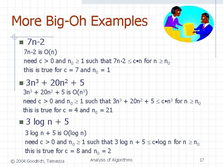
More Big-Oh Examples n 7 n-2 is O(n) need c > 0 and n 0 1 such that 7 n-2 c • n for n n 0 this is true for c = 7 and n 0 = 1 n 3 n 3 + 20 n 2 + 5 is O(n 3) need c > 0 and n 0 1 such that 3 n 3 + 20 n 2 + 5 c • n 3 for n n 0 this is true for c = 4 and n 0 = 21 n 3 log n + 5 is O(log n) need c > 0 and n 0 1 such that 3 log n + 5 c • log n for n n 0 this is true for c = 8 and n 0 = 2 © 2004 Goodrich, Tamassia Analysis of Algorithms 17

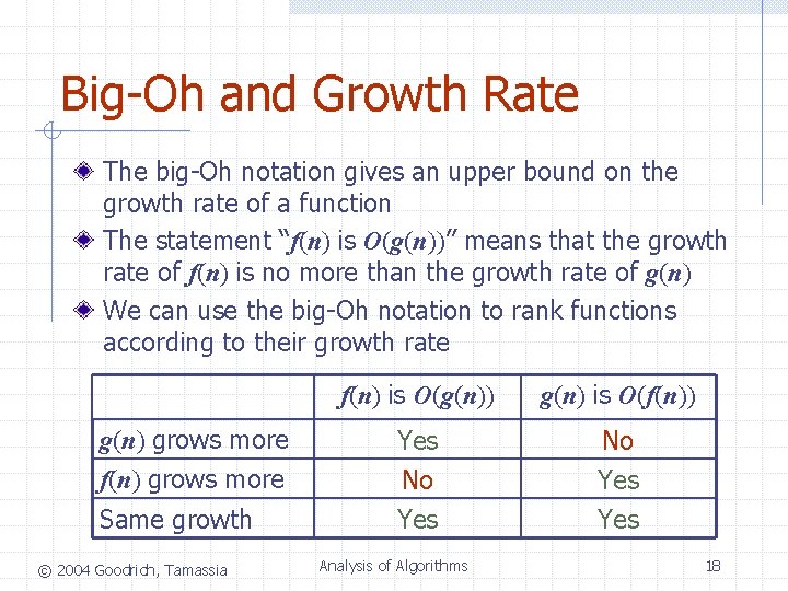
Big-Oh and Growth Rate The big-Oh notation gives an upper bound on the growth rate of a function The statement “f(n) is O(g(n))” means that the growth rate of f(n) is no more than the growth rate of g(n) We can use the big-Oh notation to rank functions according to their growth rate g(n) grows more f(n) grows more Same growth © 2004 Goodrich, Tamassia f(n) is O(g(n)) g(n) is O(f(n)) Yes No Yes Analysis of Algorithms 18

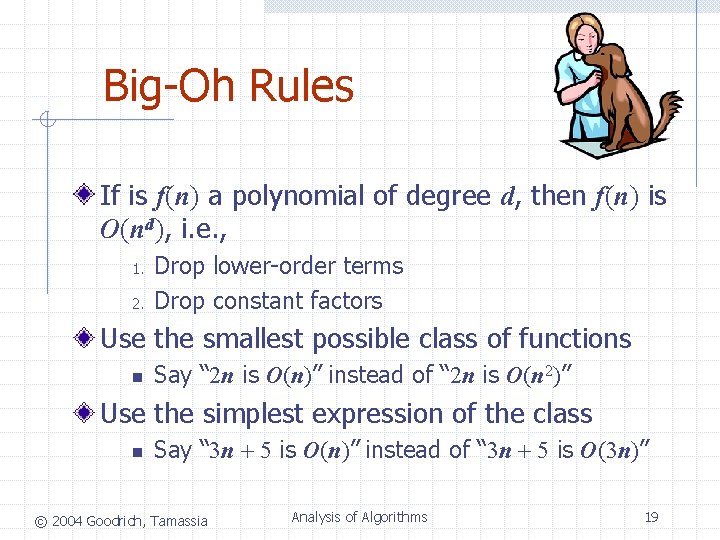
Big-Oh Rules If is f(n) a polynomial of degree d, then f(n) is O(nd), i. e. , 1. 2. Drop lower-order terms Drop constant factors Use the smallest possible class of functions n Say “ 2 n is O(n)” instead of “ 2 n is O(n 2)” Use the simplest expression of the class n Say “ 3 n + 5 is O(n)” instead of “ 3 n + 5 is O(3 n)” © 2004 Goodrich, Tamassia Analysis of Algorithms 19

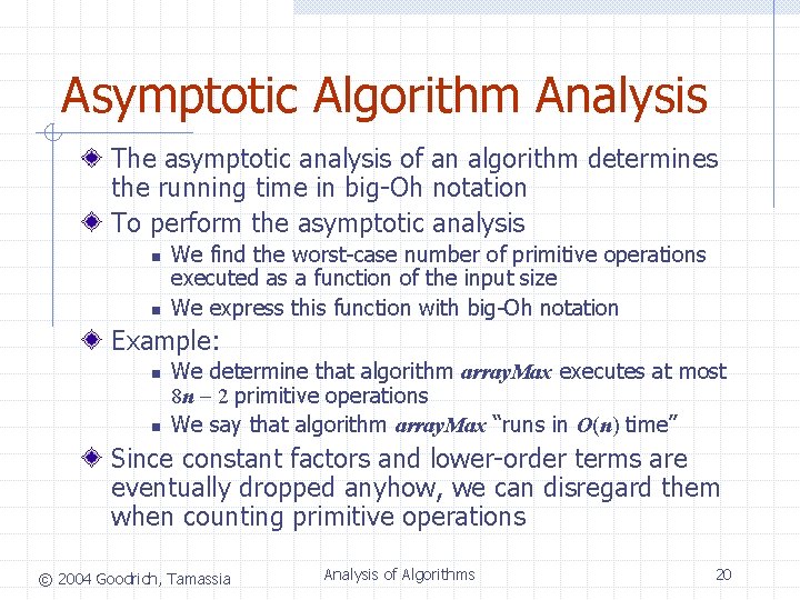
Asymptotic Algorithm Analysis The asymptotic analysis of an algorithm determines the running time in big-Oh notation To perform the asymptotic analysis n n We find the worst-case number of primitive operations executed as a function of the input size We express this function with big-Oh notation Example: n n We determine that algorithm array. Max executes at most 8 n 2 primitive operations We say that algorithm array. Max “runs in O(n) time” Since constant factors and lower-order terms are eventually dropped anyhow, we can disregard them when counting primitive operations © 2004 Goodrich, Tamassia Analysis of Algorithms 20

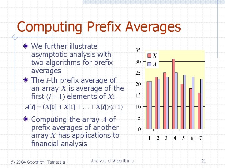
Computing Prefix Averages We further illustrate asymptotic analysis with two algorithms for prefix averages The i-th prefix average of an array X is average of the first (i + 1) elements of X: A[i] (X[0] + X[1] + … + X[i])/(i+1) Computing the array A of prefix averages of another array X has applications to financial analysis © 2004 Goodrich, Tamassia Analysis of Algorithms 21

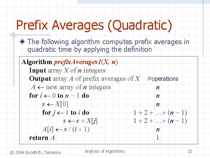
Prefix Averages (Quadratic) The following algorithm computes prefix averages in quadratic time by applying the definition Algorithm prefix. Averages 1(X, n) Input array X of n integers Output array A of prefix averages of X #operations A new array of n integers n for i 0 to n 1 do n s X[0] n for j 1 to i do 1 + 2 + …+ (n 1) s s + X[j] 1 + 2 + …+ (n 1) A[i] s / (i + 1) n return A 1 © 2004 Goodrich, Tamassia Analysis of Algorithms 22

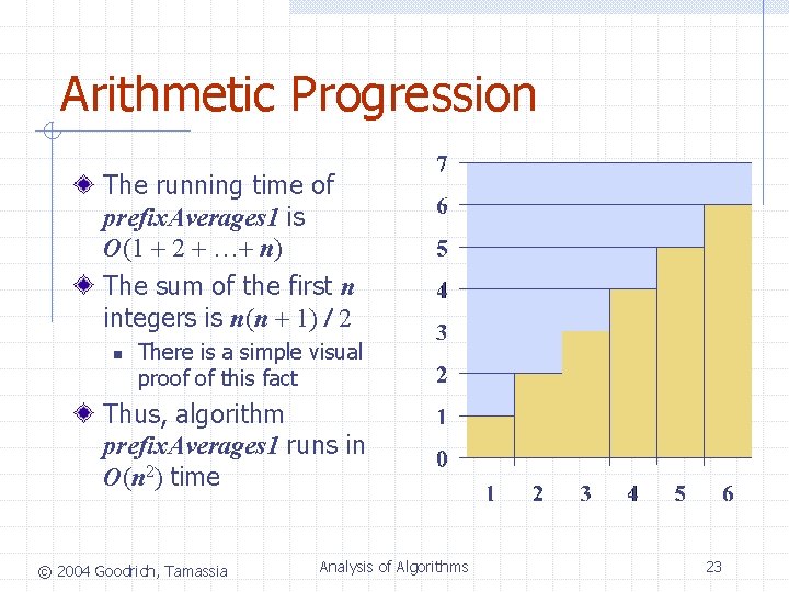
Arithmetic Progression The running time of prefix. Averages 1 is O(1 + 2 + …+ n) The sum of the first n integers is n(n + 1) / 2 n There is a simple visual proof of this fact Thus, algorithm prefix. Averages 1 runs in O(n 2) time © 2004 Goodrich, Tamassia Analysis of Algorithms 23

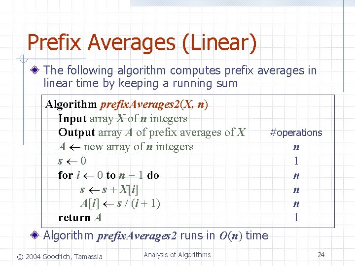
Prefix Averages (Linear) The following algorithm computes prefix averages in linear time by keeping a running sum Algorithm prefix. Averages 2(X, n) Input array X of n integers Output array A of prefix averages of X A new array of n integers s 0 for i 0 to n 1 do s s + X[i] A[i] s / (i + 1) return A #operations n 1 n n n 1 Algorithm prefix. Averages 2 runs in O(n) time © 2004 Goodrich, Tamassia Analysis of Algorithms 24

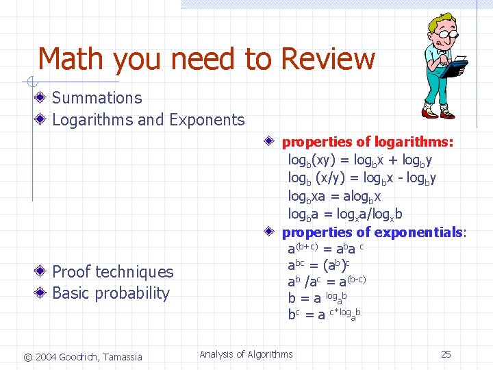
Math you need to Review Summations Logarithms and Exponents Proof techniques Basic probability © 2004 Goodrich, Tamassia properties of logarithms: logb(xy) = logbx + logby logb (x/y) = logbx - logby logbxa = alogbx logba = logxa/logxb properties of exponentials: a(b+c) = aba c abc = (ab)c ab /ac = a(b-c) b = a logab bc = a c*logab Analysis of Algorithms 25

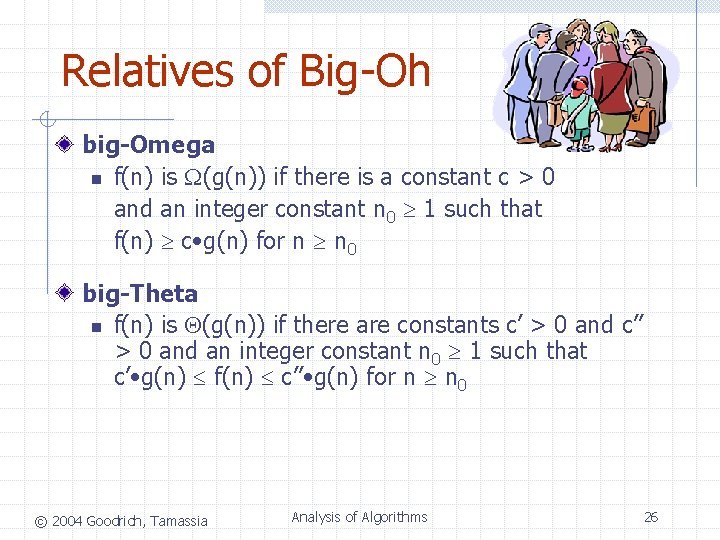
Relatives of Big-Oh big-Omega n f(n) is (g(n)) if there is a constant c > 0 and an integer constant n 0 1 such that f(n) c • g(n) for n n 0 big-Theta n f(n) is (g(n)) if there are constants c’ > 0 and c’’ > 0 and an integer constant n 0 1 such that c’ • g(n) f(n) c’’ • g(n) for n n 0 © 2004 Goodrich, Tamassia Analysis of Algorithms 26

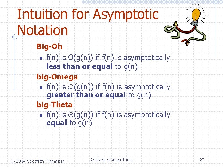
Intuition for Asymptotic Notation Big-Oh n f(n) is O(g(n)) if f(n) is asymptotically less than or equal to g(n) big-Omega n f(n) is (g(n)) if f(n) is asymptotically greater than or equal to g(n) big-Theta n f(n) is (g(n)) if f(n) is asymptotically equal to g(n) © 2004 Goodrich, Tamassia Analysis of Algorithms 27

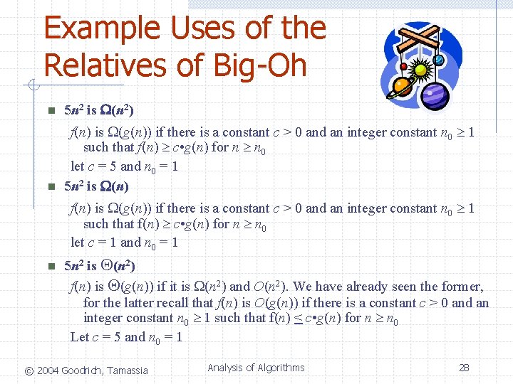
Example Uses of the Relatives of Big-Oh n 5 n 2 is (n 2) n f(n) is (g(n)) if there is a constant c > 0 and an integer constant n 0 1 such that f(n) c • g(n) for n n 0 let c = 5 and n 0 = 1 5 n 2 is (n) f(n) is (g(n)) if there is a constant c > 0 and an integer constant n 0 1 such that f(n) c • g(n) for n n 0 let c = 1 and n 0 = 1 n 5 n 2 is (n 2) f(n) is (g(n)) if it is (n 2) and O(n 2). We have already seen the former, for the latter recall that f(n) is O(g(n)) if there is a constant c > 0 and an integer constant n 0 1 such that f(n) < c • g(n) for n n 0 Let c = 5 and n 0 = 1 © 2004 Goodrich, Tamassia Analysis of Algorithms 28