STAT 497 LECTURE NOTES 4 MODEL IDENTIFICATION AND

STAT 497 LECTURE NOTES 4 MODEL IDENTIFICATION AND NONSTATIONARY TIME SERIES MODELS 1

MODEL IDENTIFICATION • We have learned a large class of linear parametric models for stationary time series processes. • Now, the question is how we can find out the best suitable model for a given observed series. How to choose the appropriate model (on order of p and q). 2

MODEL IDENTIFICATION • ACF and PACF show specific properties for specific models. Hence, we can use them as a criteria to identify the suitable model. • Using the patterns of sample ACF and sample PACF, we can identify the model. 3

MODEL SELECTION THROUGH CRITERIA • Besides s. ACF and s. PACF plots, we have also other tools for model identification. • With messy real data, s. ACF and s. PACF plots become complicated and harder to interpret. • Don’t forget to choose the best model with as few parameters as possible. • It will be seen that many different models can fit to the same data so that we should choose the most appropriate (with less parameters) one and the information criteria will help us to decide this. 4

MODEL SELECTION THROUGH CRITERIA • The three well-known information criteria are – Akaike’s information criterion (AIC) (Akaike, 1974) – Schwarz’s Bayesian Criterion (SBC) (Schwarz, 1978). Also known as Bayesian Information Criterion (BIC) – Hannan-Quinn Criteria (HQIC) (Hannan&Quinn, 1979) 5

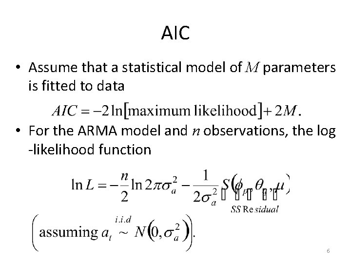
AIC • Assume that a statistical model of M parameters is fitted to data • For the ARMA model and n observations, the log -likelihood function 6

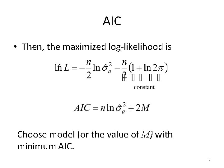
AIC • Then, the maximized log-likelihood is Choose model (or the value of M) with minimum AIC. 7

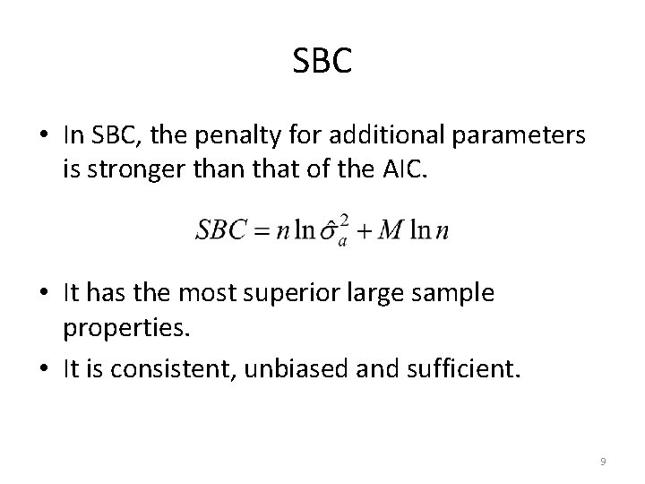
SBC • The Bayesian information criterion (BIC) or Schwarz Criterion (also SBC, SBIC) is a criterion for model selection among a class of parametric models with different numbers of parameters. • When estimating model parameters using maximum likelihood estimation, it is possible to increase the likelihood by adding additional parameters, which may result in overfitting. The BIC resolves this problem by introducing a penalty term for the number of parameters in the model. 8

SBC • In SBC, the penalty for additional parameters is stronger than that of the AIC. • It has the most superior large sample properties. • It is consistent, unbiased and sufficient. 9

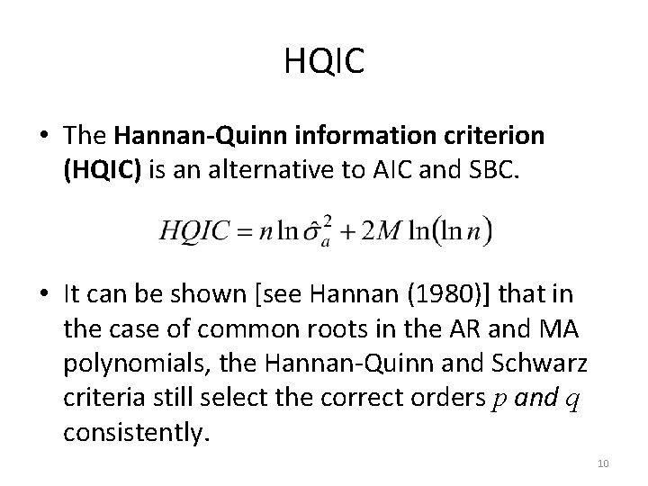
HQIC • The Hannan-Quinn information criterion (HQIC) is an alternative to AIC and SBC. • It can be shown [see Hannan (1980)] that in the case of common roots in the AR and MA polynomials, the Hannan-Quinn and Schwarz criteria still select the correct orders p and q consistently. 10

THE INVERSE AUTOCORRELATION FUNCTION • The sample inverse autocorrelation function (SIACF) plays much the same role in ARIMA modeling as the sample partial autocorrelation function (SPACF), but it generally indicates subset and seasonal autoregressive models better than the SPACF. 11

THE INVERSE AUTOCORRELATION FUNCTION • Additionally, the SIACF can be useful for detecting over-differencing. If the data come from a nonstationary or nearly nonstationary model, the SIACF has the characteristics of a noninvertible moving-average. Likewise, if the data come from a model with a noninvertible moving average, then the SIACF has nonstationary characteristics and therefore decays slowly. In particular, if the data have been over-differenced, the SIACF looks like a SACF from a nonstationary process 12

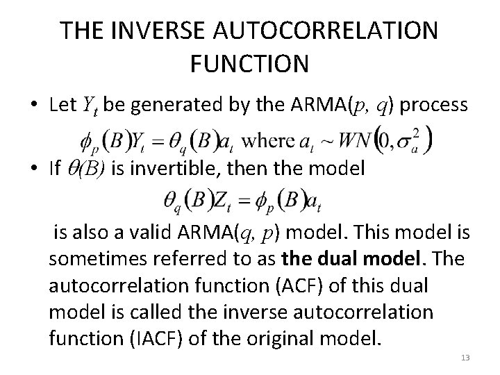
THE INVERSE AUTOCORRELATION FUNCTION • Let Yt be generated by the ARMA(p, q) process • If (B) is invertible, then the model is also a valid ARMA(q, p) model. This model is sometimes referred to as the dual model. The autocorrelation function (ACF) of this dual model is called the inverse autocorrelation function (IACF) of the original model. 13

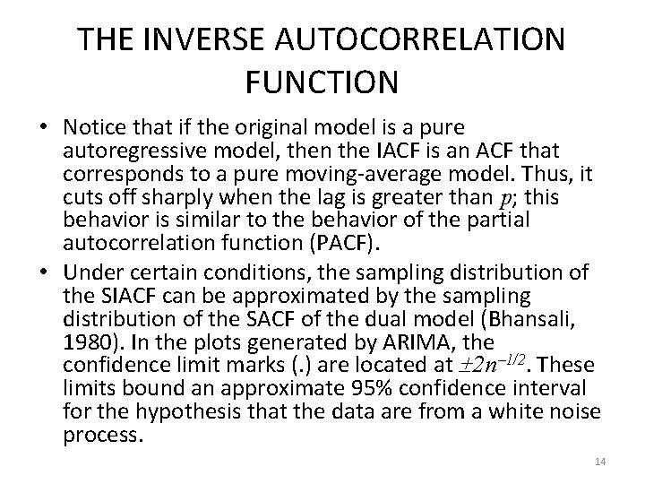
THE INVERSE AUTOCORRELATION FUNCTION • Notice that if the original model is a pure autoregressive model, then the IACF is an ACF that corresponds to a pure moving-average model. Thus, it cuts off sharply when the lag is greater than p; this behavior is similar to the behavior of the partial autocorrelation function (PACF). • Under certain conditions, the sampling distribution of the SIACF can be approximated by the sampling distribution of the SACF of the dual model (Bhansali, 1980). In the plots generated by ARIMA, the confidence limit marks (. ) are located at 2 n 1/2. These limits bound an approximate 95% confidence interval for the hypothesis that the data are from a white noise process. 14

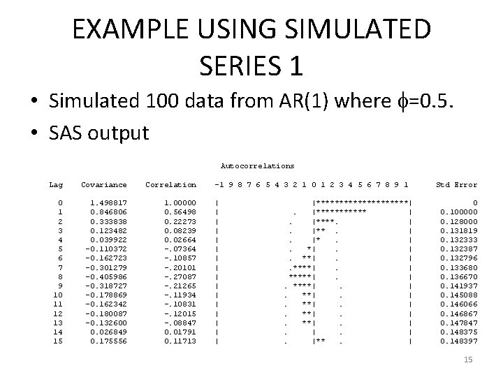
EXAMPLE USING SIMULATED SERIES 1 • Simulated 100 data from AR(1) where =0. 5. • SAS output Autocorrelations Lag Covariance Correlation 0 1 2 3 4 5 6 7 8 9 10 11 12 13 14 15 1. 498817 0. 846806 0. 333838 0. 123482 0. 039922 -0. 110372 -0. 162723 -0. 301279 -0. 405986 -0. 318727 -0. 178869 -0. 162342 -0. 180087 -0. 132600 0. 026849 0. 175556 1. 00000 0. 56498 0. 22273 0. 08239 0. 02664 -. 07364 -. 10857 -. 20101 -. 27087 -. 21265 -. 11934 -. 10831 -. 12015 -. 08847 0. 01791 0. 11713 -1 9 8 7 6 5 4 3 2 1 0 1 2 3 4 5 6 7 8 9 1 | | | | |**********| |****** |. |****. |. |*. |. *|. |. ****|. | *****|. |. |**. |. Std Error 0 0. 100000 0. 128000 0. 131819 0. 132333 0. 132387 0. 132796 0. 133680 0. 136670 0. 141937 0. 145088 0. 146066 0. 146867 0. 147847 0. 148375 0. 148397 15

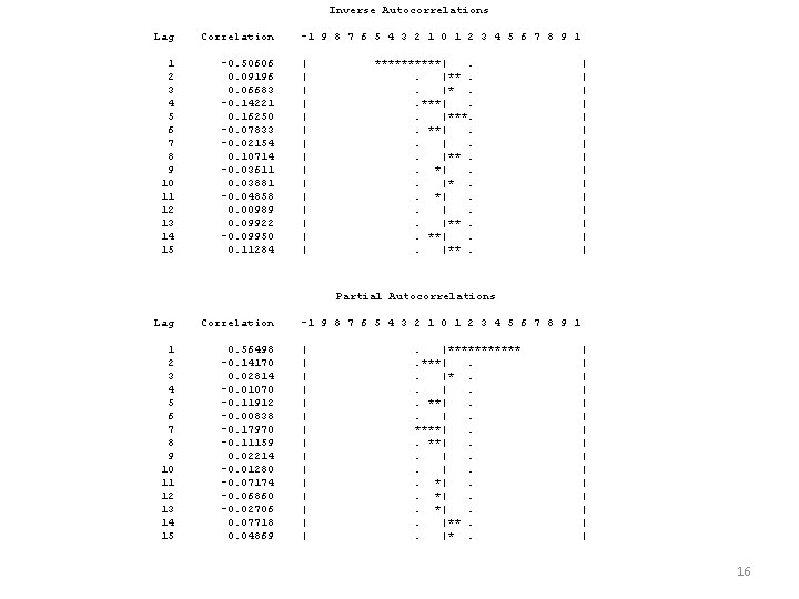
Inverse Autocorrelations Lag Correlation 1 2 3 4 5 6 7 8 9 10 11 12 13 14 15 -0. 50606 0. 09196 0. 06683 -0. 14221 0. 16250 -0. 07833 -0. 02154 0. 10714 -0. 03611 0. 03881 -0. 04858 0. 00989 0. 09922 -0. 09950 0. 11284 -1 9 8 7 6 5 4 3 2 1 0 1 2 3 4 5 6 7 8 9 1 | | | | *****|. . |**. . |*. . ***|. . |***. . **|. . |**. . *|. . |**. . **|. . |**. | | | | Partial Autocorrelations Lag Correlation 1 2 3 4 5 6 7 8 9 10 11 12 13 14 15 0. 56498 -0. 14170 0. 02814 -0. 01070 -0. 11912 -0. 00838 -0. 17970 -0. 11159 0. 02214 -0. 01280 -0. 07174 -0. 06860 -0. 02706 0. 07718 0. 04869 -1 9 8 7 6 5 4 3 2 1 0 1 2 3 4 5 6 7 8 9 1 | | | | . |******. ***|. . |*. . |. . **|. . |. ****|. . *|. . |**. . |*. | | | | 16

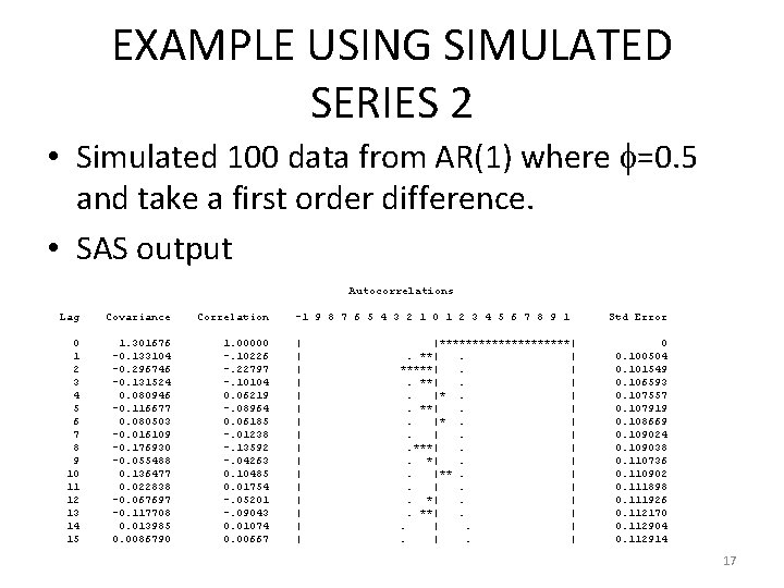
EXAMPLE USING SIMULATED SERIES 2 • Simulated 100 data from AR(1) where =0. 5 and take a first order difference. • SAS output Autocorrelations Lag Covariance Correlation 0 1 2 3 4 5 6 7 8 9 10 11 12 13 14 15 1. 301676 -0. 133104 -0. 296746 -0. 131524 0. 080946 -0. 116677 0. 080503 -0. 016109 -0. 176930 -0. 055488 0. 136477 0. 022838 -0. 067697 -0. 117708 0. 013985 0. 0086790 1. 00000 -. 10226 -. 22797 -. 10104 0. 06219 -. 08964 0. 06185 -. 01238 -. 13592 -. 04263 0. 10485 0. 01754 -. 05201 -. 09043 0. 01074 0. 00667 -1 9 8 7 6 5 4 3 2 1 0 1 2 3 4 5 6 7 8 9 1 | | | | |**********|. | *****|. |. |*. |. |. |. ***|. |. |**. |. |. |. **|. | Std Error 0 0. 100504 0. 101549 0. 106593 0. 107557 0. 107919 0. 108669 0. 109024 0. 109038 0. 110736 0. 110902 0. 111898 0. 111926 0. 112170 0. 112904 0. 112914 17

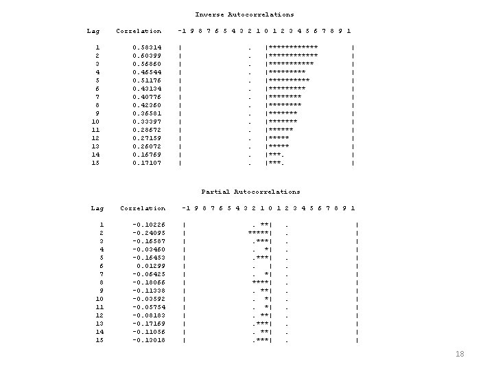
Inverse Autocorrelations Lag Correlation 1 2 3 4 5 6 7 8 9 10 11 12 13 14 15 0. 58314 0. 60399 0. 56860 0. 46544 0. 51176 0. 43134 0. 40776 0. 42360 0. 36581 0. 33397 0. 28672 0. 27159 0. 26072 0. 16769 0. 17107 -1 9 8 7 6 5 4 3 2 1 0 1 2 3 4 5 6 7 8 9 1 | | | | . . . . |************ |********** |******** |******* |***** |***. | | | | Partial Autocorrelations Lag Correlation 1 2 3 4 5 6 7 8 9 10 11 12 13 14 15 -0. 10226 -0. 24095 -0. 16587 -0. 03460 -0. 16453 0. 01299 -0. 06425 -0. 18066 -0. 11338 -0. 03592 -0. 05754 -0. 08183 -0. 17169 -0. 11056 -0. 13018 -1 9 8 7 6 5 4 3 2 1 0 1 2 3 4 5 6 7 8 9 1 | | | | . **| *****|. *|. ***|. |. *| ****|. *|. **|. ***| . . . . | | | | 18

THE EXTENDED SAMPLE AUTOCORRELATION FUNCTION_ESACF • The extended sample autocorrelation function (ESACF) method can tentatively identify the orders of a stationary or nonstationary ARMA process based on iterated least squares estimates of the autoregressive parameters. Tsay and Tiao (1984) proposed the technique. 19

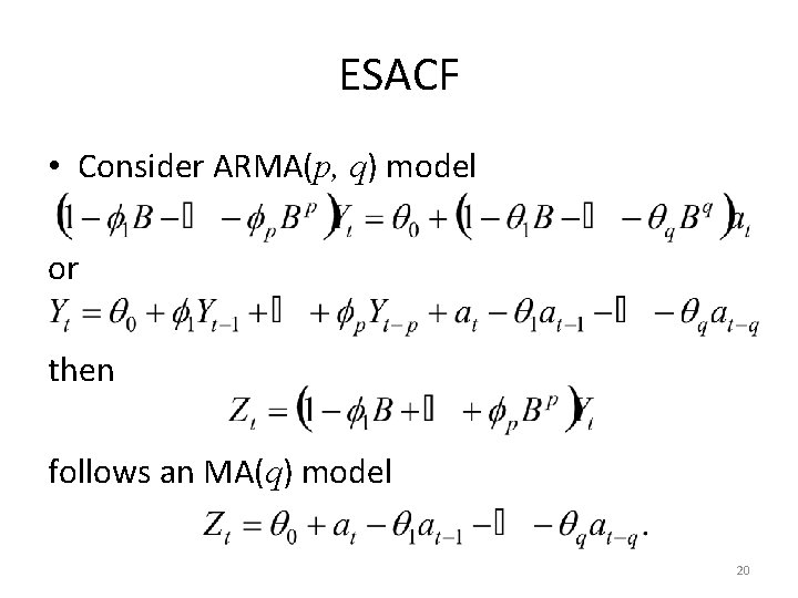
ESACF • Consider ARMA(p, q) model or then follows an MA(q) model 20

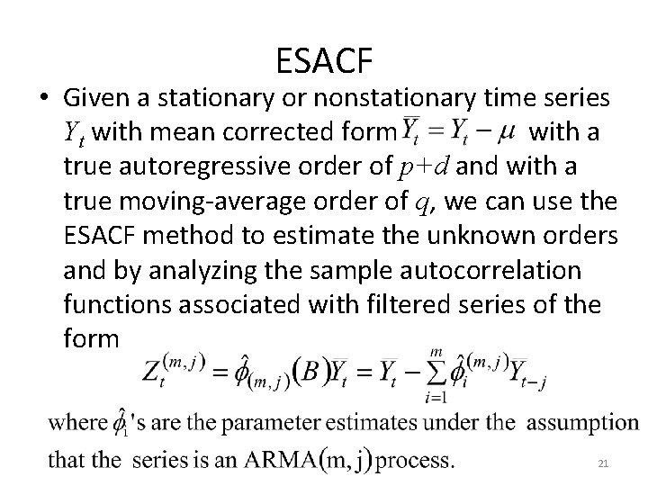
ESACF • Given a stationary or nonstationary time series Yt with mean corrected form with a true autoregressive order of p+d and with a true moving-average order of q, we can use the ESACF method to estimate the unknown orders and by analyzing the sample autocorrelation functions associated with filtered series of the form 21

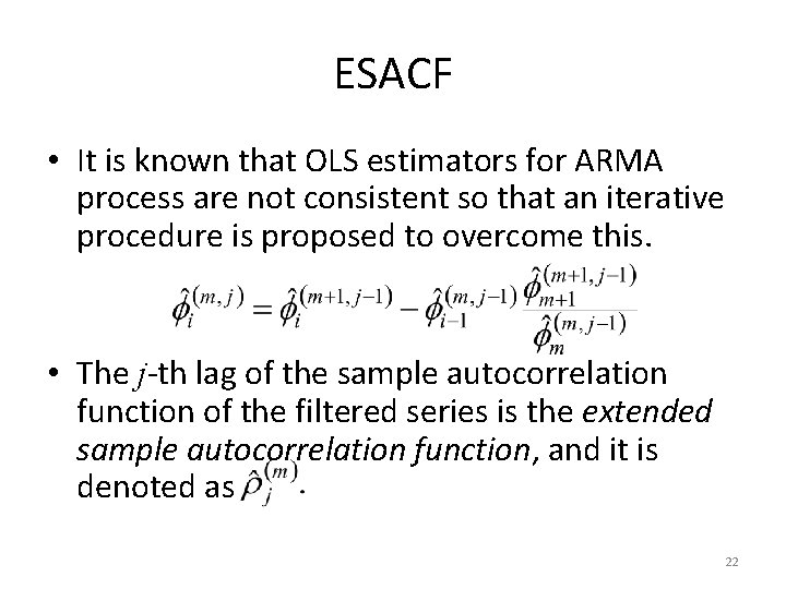
ESACF • It is known that OLS estimators for ARMA process are not consistent so that an iterative procedure is proposed to overcome this. • The j-th lag of the sample autocorrelation function of the filtered series is the extended sample autocorrelation function, and it is denoted as 22

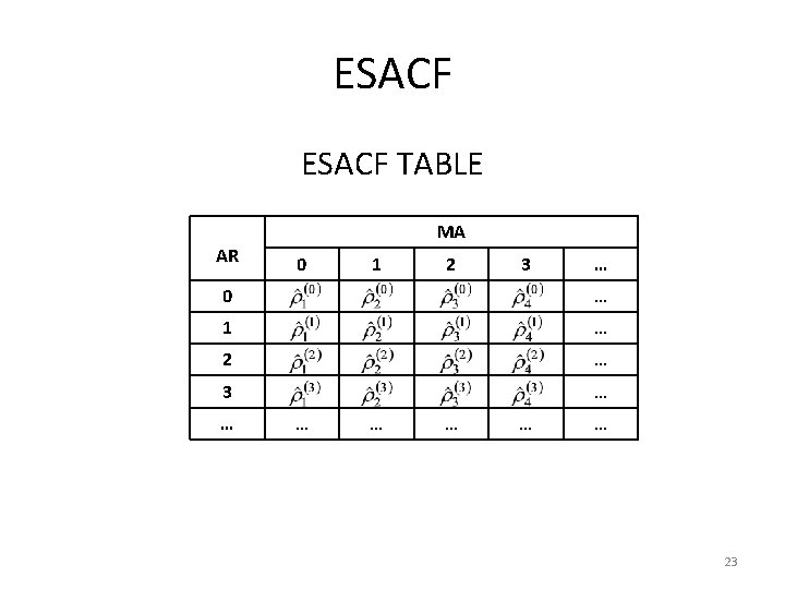
ESACF TABLE AR MA 0 1 2 3 … 0 … 1 … 2 … 3 … … … … 23

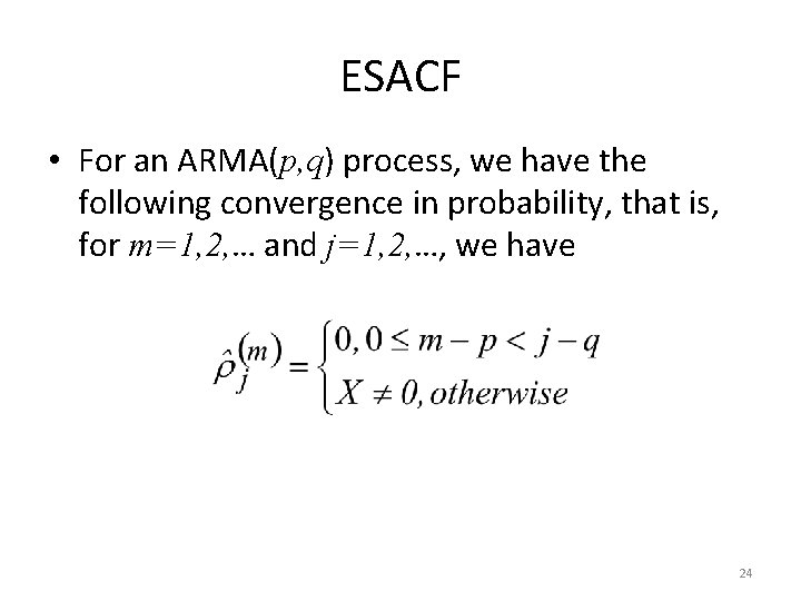
ESACF • For an ARMA(p, q) process, we have the following convergence in probability, that is, for m=1, 2, … and j=1, 2, …, we have 24

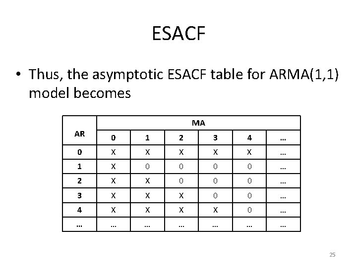
ESACF • Thus, the asymptotic ESACF table for ARMA(1, 1) model becomes MA AR 0 1 2 3 4 … 0 X X X … 1 X 0 0 … 2 X X 0 0 0 … 3 X X X 0 0 … 4 X X 0 … … … … 25

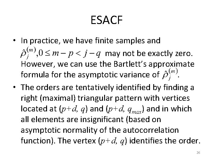
ESACF • In practice, we have finite samples and may not be exactly zero. However, we can use the Bartlett’s approximate formula for the asymptotic variance of. • The orders are tentatively identified by finding a right (maximal) triangular pattern with vertices located at (p+d, q) and (p+d, qmax) and in which all elements are insignificant (based on asymptotic normality of the autocorrelation function). The vertex (p+d, q) identifies the order. 26

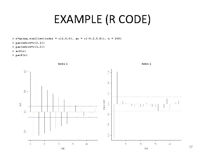
EXAMPLE (R CODE) > > > x=arima. sim(list(order = c(2, 0, 0), ar = c(-0. 2, 0. 6)), n = 200) par(mfrow=c(2, 1)) par(mfrow=c(1, 2)) acf(x) pacf(x) 27

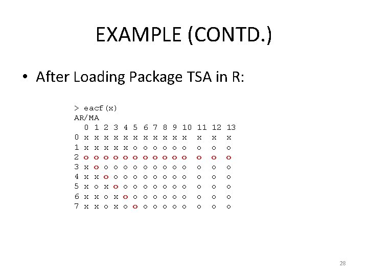
EXAMPLE (CONTD. ) • After Loading Package TSA in R: > eacf(x) AR/MA 0 1 2 3 0 x x 1 x x 2 o o 3 x o o o 4 x x o o 5 x o 6 x x o x 7 x x o x 4 x x o o o 5 x o o o o 6 x o o o o 7 x o o o o 8 x o o o o 9 x o o o o 10 x o o o o 11 x o o o o 12 x o o o o 13 x o o o o 28

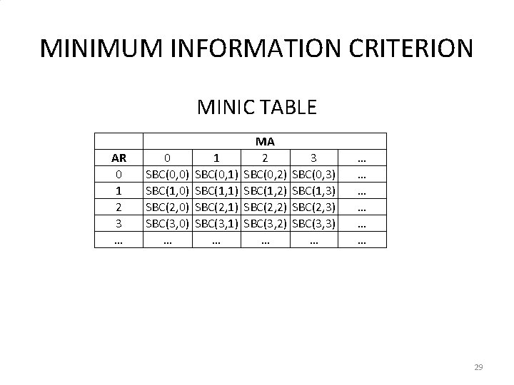
MINIMUM INFORMATION CRITERION MINIC TABLE AR 0 1 2 3 … 0 SBC(0, 0) SBC(1, 0) SBC(2, 0) SBC(3, 0) … 1 SBC(0, 1) SBC(1, 1) SBC(2, 1) SBC(3, 1) … MA 2 SBC(0, 2) SBC(1, 2) SBC(2, 2) SBC(3, 2) … 3 SBC(0, 3) SBC(1, 3) SBC(2, 3) SBC(3, 3) … … … … 29

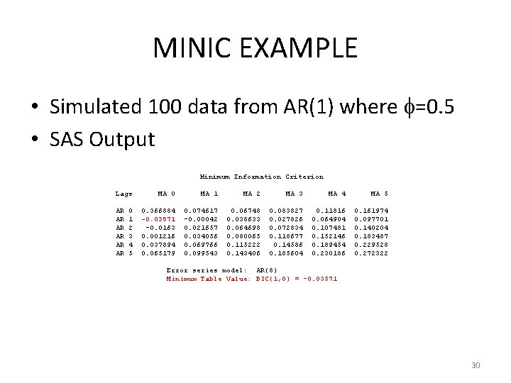
MINIC EXAMPLE • Simulated 100 data from AR(1) where =0. 5 • SAS Output Minimum Information Criterion Lags AR AR AR 0 1 2 3 4 5 MA 0 MA 1 MA 2 MA 3 MA 4 MA 5 0. 366884 -0. 03571 -0. 0163 0. 001216 0. 037894 0. 065179 0. 074617 -0. 00042 0. 021657 0. 034056 0. 069766 0. 099543 0. 06748 0. 038633 0. 064698 0. 080065 0. 115222 0. 143406 0. 083827 0. 027826 0. 072834 0. 118677 0. 14586 0. 185604 0. 11816 0. 064904 0. 107481 0. 152146 0. 189454 0. 230186 0. 161974 0. 097701 0. 140204 0. 183487 0. 229528 0. 272322 Error series model: AR(8) Minimum Table Value: BIC(1, 0) = -0. 03571 30

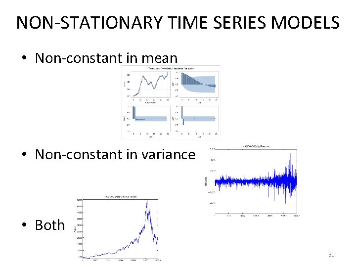
NON-STATIONARY TIME SERIES MODELS • Non-constant in mean • Non-constant in variance • Both 31

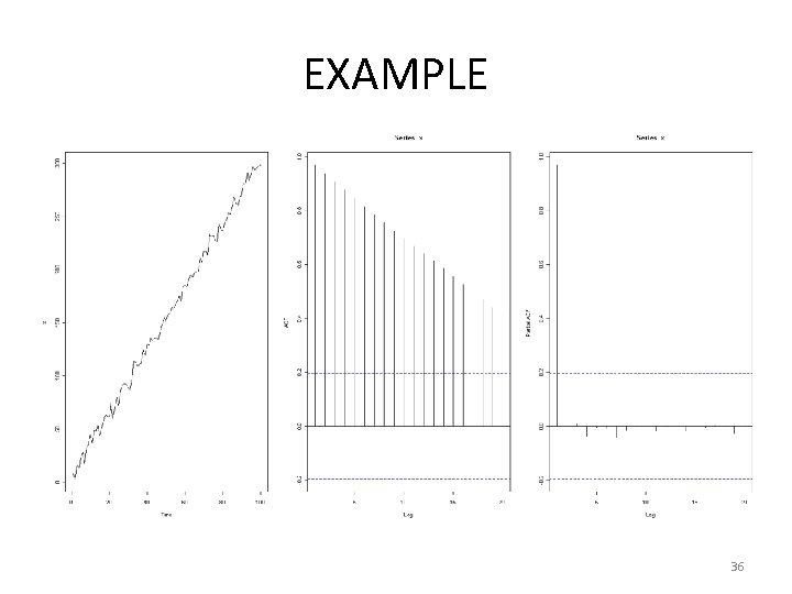
NON-STATIONARY TIME SERIES MODELS • Inspection of the ACF serves as a rough indicator of whether a trend is present in a series. A slow decay in ACF is indicative of a large characteristic root; a true unit root process, or a trend stationary process. • Formal tests can help to determine whether a system contains a trend and whether the trend is deterministic or stochastic. 32

NON-STATIONARITY IN MEAN • Deterministic trend – Detrending • Stochastic trend – Differencing 33

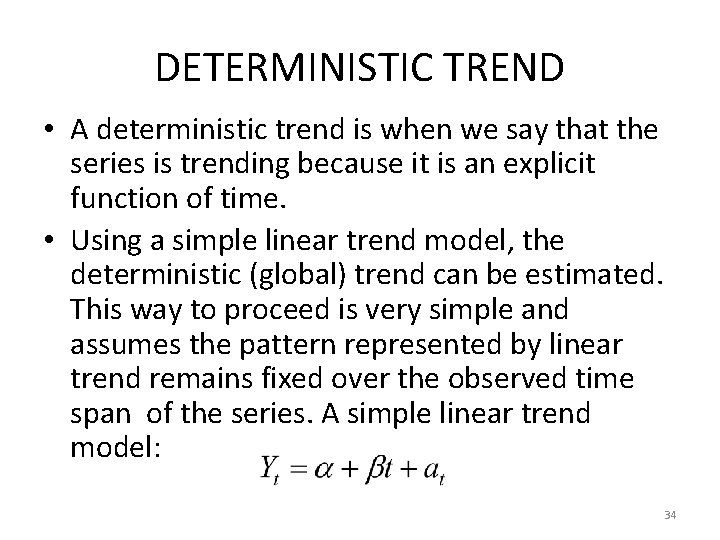
DETERMINISTIC TREND • A deterministic trend is when we say that the series is trending because it is an explicit function of time. • Using a simple linear trend model, the deterministic (global) trend can be estimated. This way to proceed is very simple and assumes the pattern represented by linear trend remains fixed over the observed time span of the series. A simple linear trend model: 34

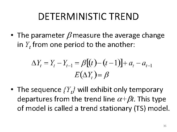
DETERMINISTIC TREND • The parameter measure the average change in Yt from one period to the another: • The sequence {Yt} will exhibit only temporary departures from the trend line + t. This type of model is called a trend stationary (TS) model. 35

EXAMPLE 36

TREND STATIONARY • If a series has a deterministic time trend, then we simply regress Yt on an intercept and a time trend (t=1, 2, …, n) and save the residuals. The residuals are detrended series. If Yt is stochastic, we do not necessarily get stationary series. 37

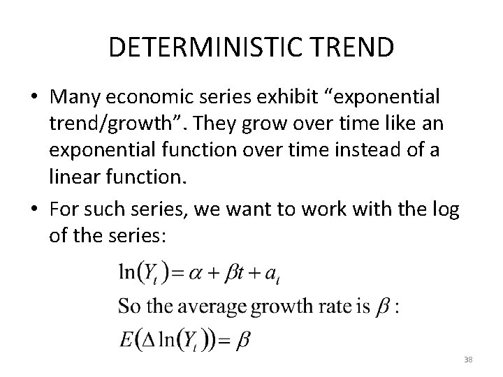
DETERMINISTIC TREND • Many economic series exhibit “exponential trend/growth”. They grow over time like an exponential function over time instead of a linear function. • For such series, we want to work with the log of the series: 38

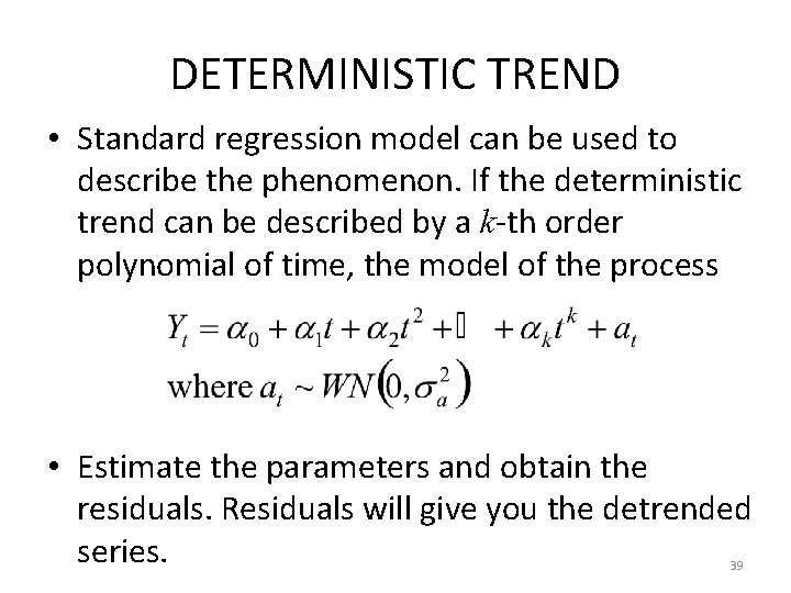
DETERMINISTIC TREND • Standard regression model can be used to describe the phenomenon. If the deterministic trend can be described by a k-th order polynomial of time, the model of the process • Estimate the parameters and obtain the residuals. Residuals will give you the detrended series. 39

DETERMINISTIC TREND • This model has a short memory. • If a shock hits a series, it goes back to trend level in short time. Hence, the best forecasts are not affected. • Rarely model like this is useful in practice. A more realistic model involves stochastic (local) trend. 40

STOCHASTIC TREND • A more modern approach is to consider trends in time series as a variable. A variable trend exists when a trend changes in an unpredictable way. Therefore, it is considered as stochastic. 41

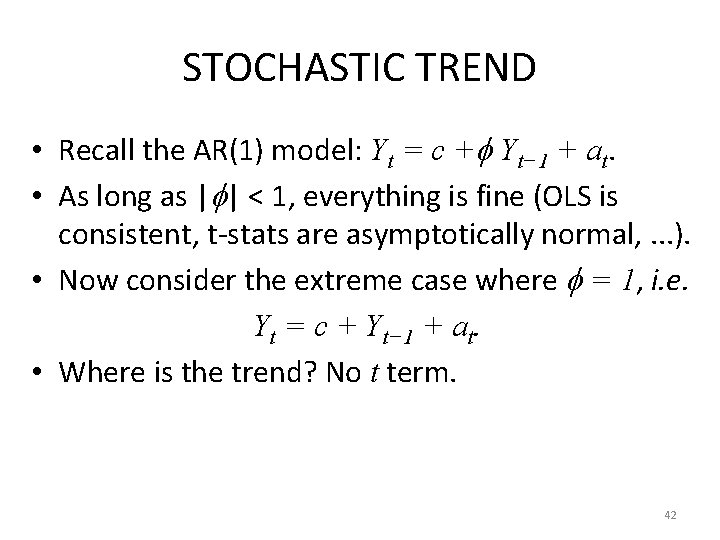
STOCHASTIC TREND • Recall the AR(1) model: Yt = c + Yt− 1 + at. • As long as | | < 1, everything is fine (OLS is consistent, t-stats are asymptotically normal, . . . ). • Now consider the extreme case where = 1, i. e. Yt = c + Yt− 1 + at. • Where is the trend? No t term. 42

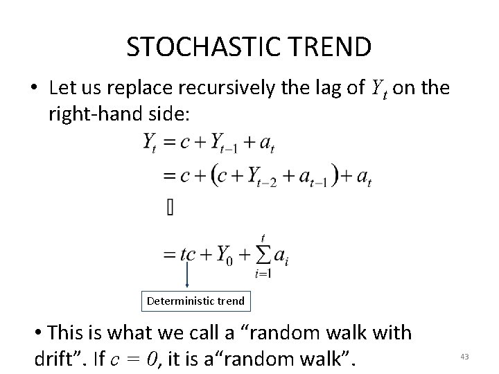
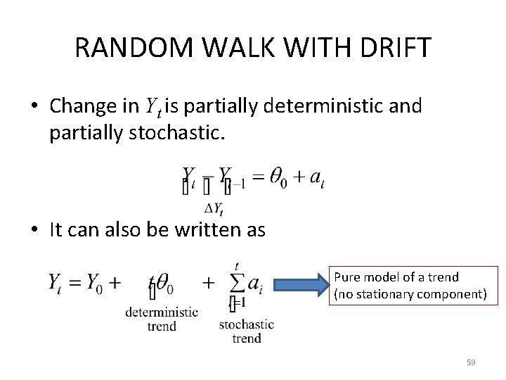
STOCHASTIC TREND • Let us replace recursively the lag of Yt on the right-hand side: Deterministic trend • This is what we call a “random walk with drift”. If c = 0, it is a“random walk”. 43

STOCHASTIC TREND • Each ai shock represents shift in the intercept. Since all values of {ai} have a coefficient of unity, the effect of each shock on the intercept term is permanent. • In the time series literature, such a sequence is said to have a stochastic trend since each ai shock imparts a permanent and random change in the conditional mean of the series. To be able to define this situation, we use Autoregressive Integrated Moving Average (ARIMA) models. 44

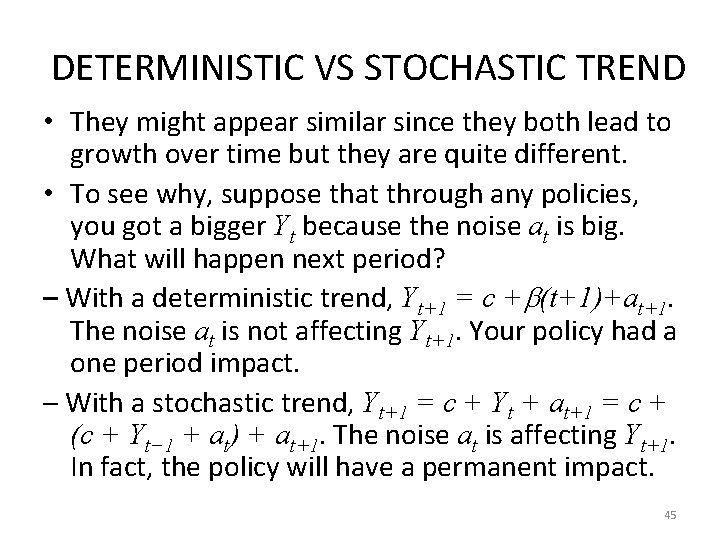
DETERMINISTIC VS STOCHASTIC TREND • They might appear similar since they both lead to growth over time but they are quite different. • To see why, suppose that through any policies, you got a bigger Yt because the noise at is big. What will happen next period? – With a deterministic trend, Yt+1 = c + (t+1)+at+1. The noise at is not affecting Yt+1. Your policy had a one period impact. – With a stochastic trend, Yt+1 = c + Yt + at+1 = c + (c + Yt− 1 + at) + at+1. The noise at is affecting Yt+1. In fact, the policy will have a permanent impact. 45

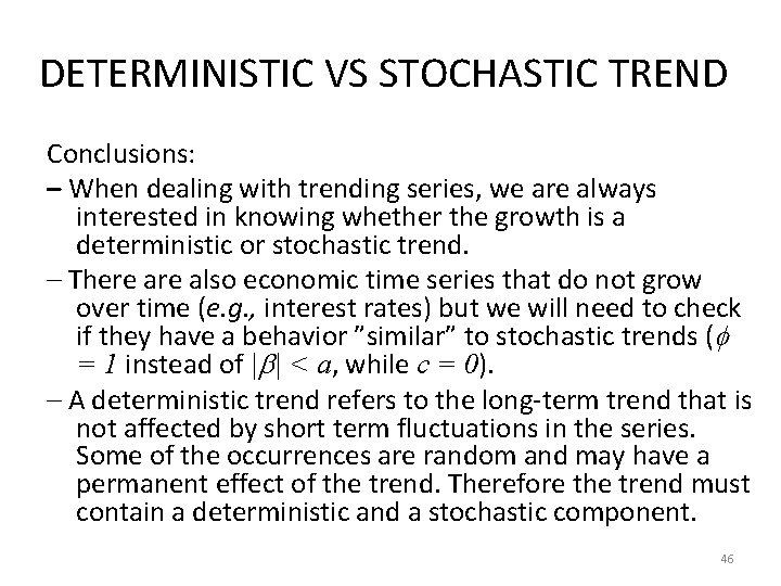
DETERMINISTIC VS STOCHASTIC TREND Conclusions: – When dealing with trending series, we are always interested in knowing whether the growth is a deterministic or stochastic trend. – There also economic time series that do not grow over time (e. g. , interest rates) but we will need to check if they have a behavior ”similar” to stochastic trends ( = 1 instead of | | < a, while c = 0). – A deterministic trend refers to the long-term trend that is not affected by short term fluctuations in the series. Some of the occurrences are random and may have a permanent effect of the trend. Therefore the trend must contain a deterministic and a stochastic component. 46

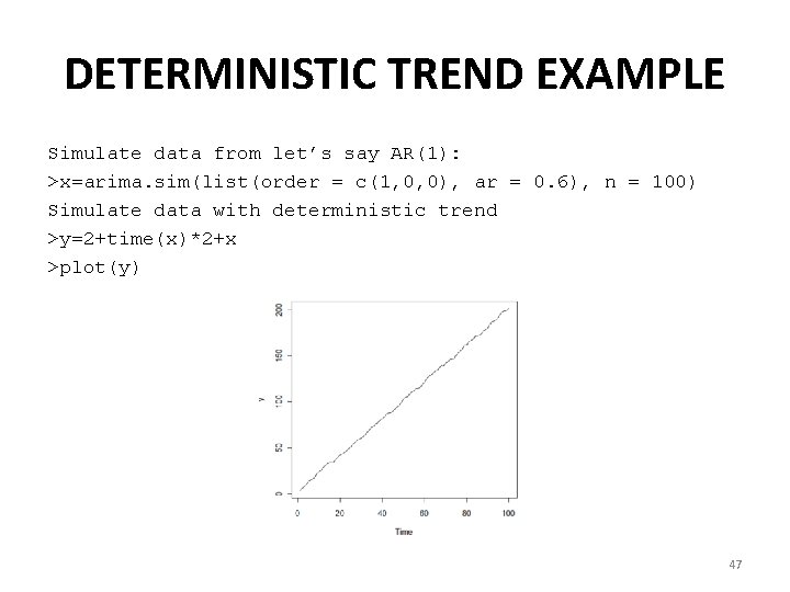
DETERMINISTIC TREND EXAMPLE Simulate data from let’s say AR(1): >x=arima. sim(list(order = c(1, 0, 0), ar = 0. 6), n = 100) Simulate data with deterministic trend >y=2+time(x)*2+x >plot(y) 47

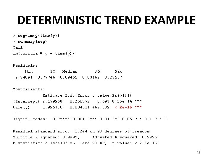
DETERMINISTIC TREND EXAMPLE > reg=lm(y~time(y)) > summary(reg) Call: lm(formula = y ~ time(y)) Residuals: Min 1 Q Median -2. 74091 -0. 77746 -0. 09465 3 Q 0. 83162 Max 3. 27567 Coefficients: Estimate Std. Error t value Pr(>|t|) (Intercept) 2. 179968 0. 250772 8. 693 8. 25 e-14 *** time(y) 1. 995380 0. 004311 462. 839 < 2 e-16 *** --Signif. codes: 0 ‘***’ 0. 001 ‘**’ 0. 01 ‘*’ 0. 05 ‘. ’ 0. 1 ‘ ’ 1 Residual standard error: 1. 244 on 98 degrees of freedom Multiple R-squared: 0. 9995, Adjusted R-squared: 0. 9995 F-statistic: 2. 142 e+05 on 1 and 98 DF, p-value: < 2. 2 e-16 48

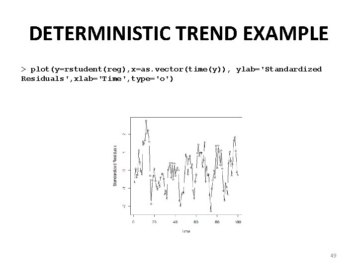
DETERMINISTIC TREND EXAMPLE > plot(y=rstudent(reg), x=as. vector(time(y)), ylab='Standardized Residuals', xlab='Time', type='o') 49

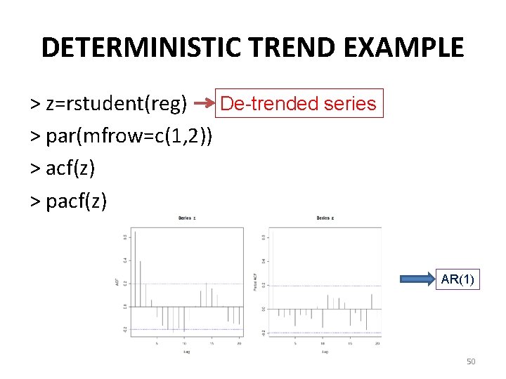
DETERMINISTIC TREND EXAMPLE > z=rstudent(reg) De-trended series > par(mfrow=c(1, 2)) > acf(z) > pacf(z) AR(1) 50

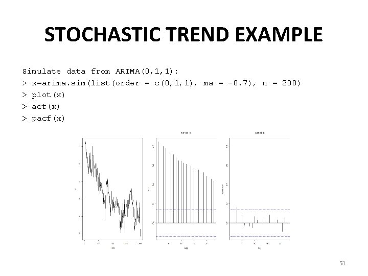
STOCHASTIC TREND EXAMPLE Simulate data from ARIMA(0, 1, 1): > x=arima. sim(list(order = c(0, 1, 1), ma = -0. 7), n = 200) > plot(x) > acf(x) > pacf(x) 51

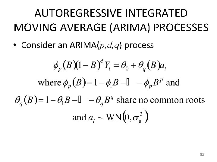
AUTOREGRESSIVE INTEGRATED MOVING AVERAGE (ARIMA) PROCESSES • Consider an ARIMA(p, d, q) process 52

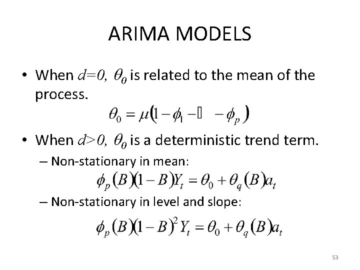
ARIMA MODELS • When d=0, 0 is related to the mean of the process. • When d>0, 0 is a deterministic trend term. – Non-stationary in mean: – Non-stationary in level and slope: 53

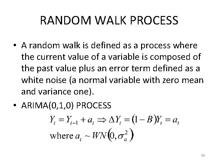
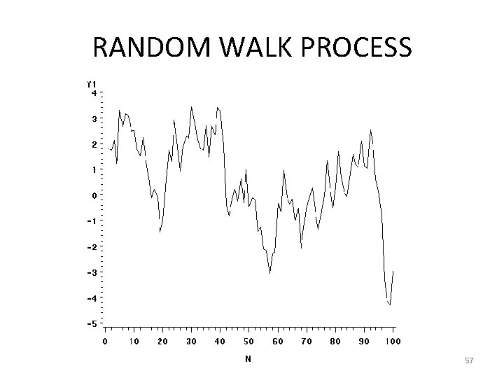
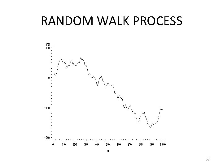
RANDOM WALK PROCESS • A random walk is defined as a process where the current value of a variable is composed of the past value plus an error term defined as a white noise (a normal variable with zero mean and variance one). • ARIMA(0, 1, 0) PROCESS 54

RANDOM WALK PROCESS • • Behavior of stock market. Brownian motion. Movement of a drunken men. It is a limiting process of AR(1). 55

RANDOM WALK PROCESS • The implication of a process of this type is that the best prediction of Y for next period is the current value, or in other words the process does not allow to predict the change (Yt Yt-1). That is, the change of Y is absolutely random. • It can be shown that the mean of a random walk process is constant but its variance is not. Therefore a random walk process is nonstationary, and its variance increases with t. • In practice, the presence of a random walk process makes the forecast process very simple since all the future values of Yt+s for s > 0, is simply Yt. 56

RANDOM WALK PROCESS 57

RANDOM WALK PROCESS 58

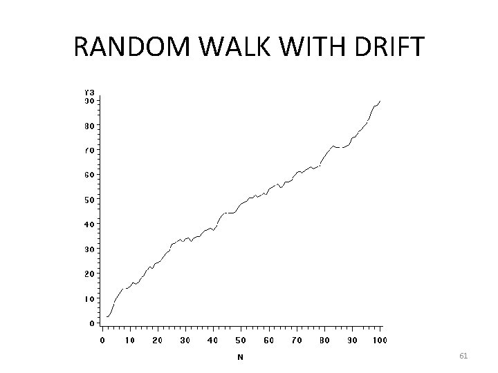
RANDOM WALK WITH DRIFT • Change in Yt is partially deterministic and partially stochastic. • It can also be written as Pure model of a trend (no stationary component) 59

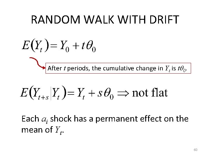
RANDOM WALK WITH DRIFT After t periods, the cumulative change in Yt is t 0. Each ai shock has a permanent effect on the mean of Yt. 60

RANDOM WALK WITH DRIFT 61

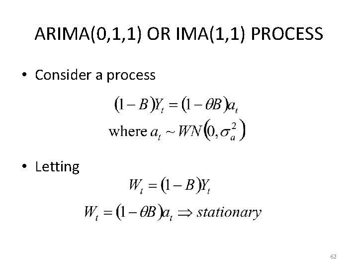
ARIMA(0, 1, 1) OR IMA(1, 1) PROCESS • Consider a process • Letting 62

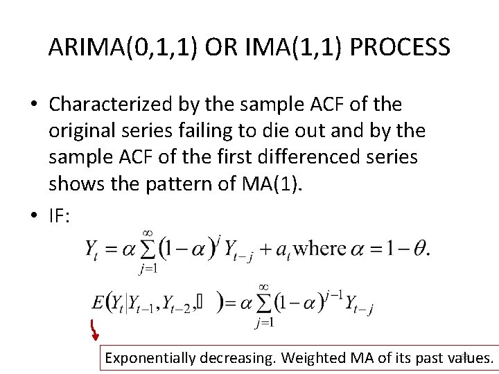
ARIMA(0, 1, 1) OR IMA(1, 1) PROCESS • Characterized by the sample ACF of the original series failing to die out and by the sample ACF of the first differenced series shows the pattern of MA(1). • IF: 63 Exponentially decreasing. Weighted MA of its past values.

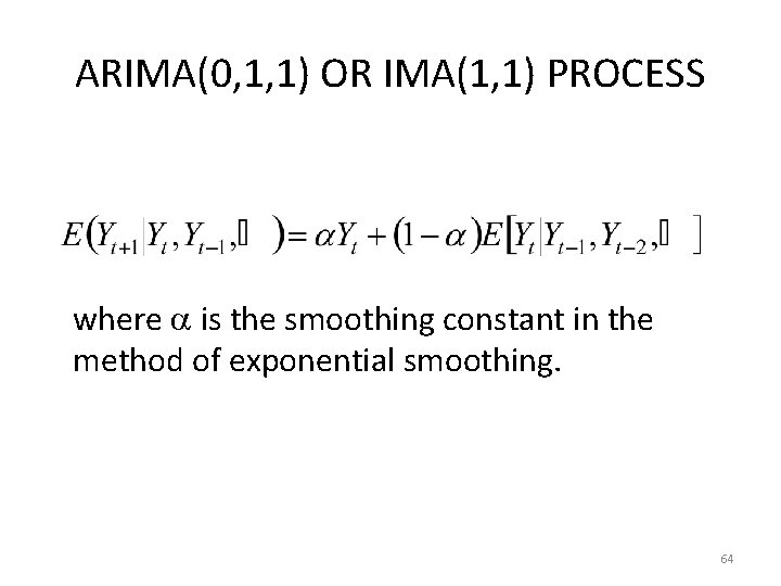
ARIMA(0, 1, 1) OR IMA(1, 1) PROCESS where is the smoothing constant in the method of exponential smoothing. 64

REMOVING THE TREND • Shocks to a stationary time series are temporary over time. The series revert to its long-run mean. • A series containing a trend will not revert to a long-run mean. The usual methods for eliminating the trend are detrending and differencing. 65

DETRENDING • Detrending is used to remove deterministic trend. • Regress Yt on time and save the residuals. • Then, check whether residuals are stationary. 66

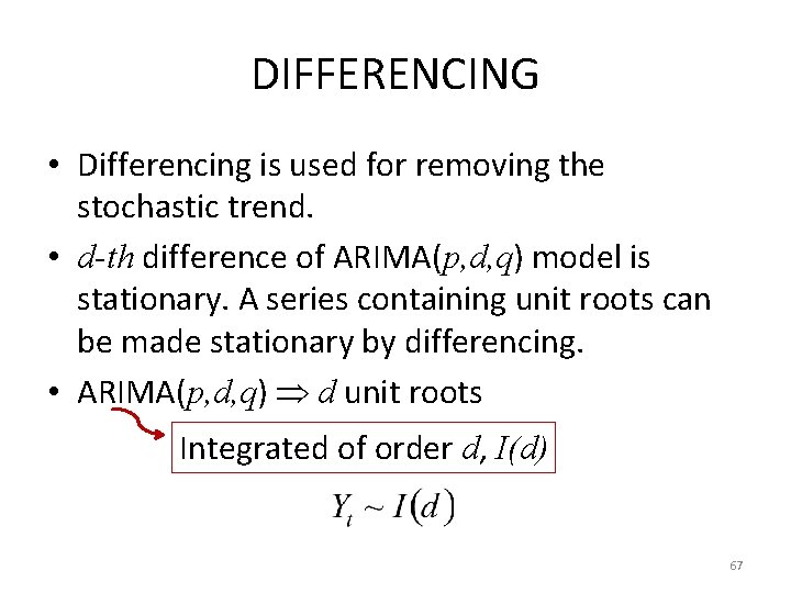
DIFFERENCING • Differencing is used for removing the stochastic trend. • d-th difference of ARIMA(p, d, q) model is stationary. A series containing unit roots can be made stationary by differencing. • ARIMA(p, d, q) d unit roots Integrated of order d, I(d) 67

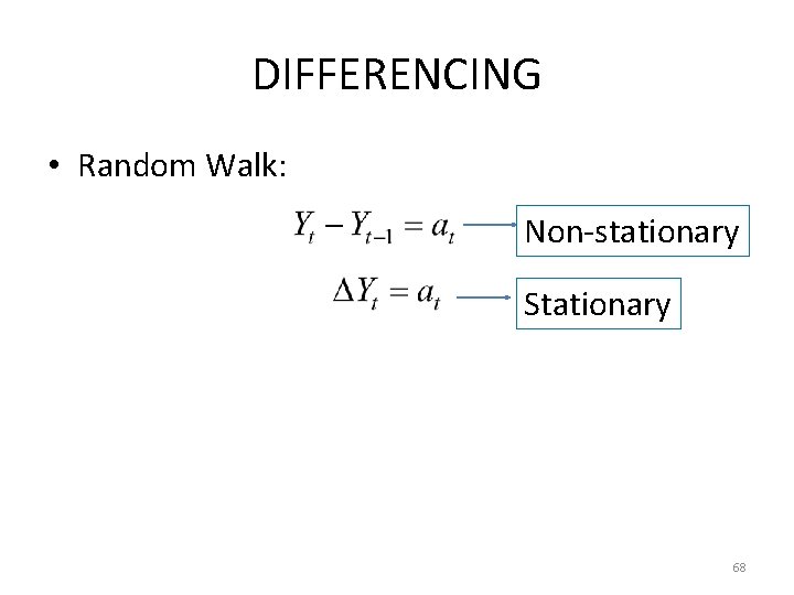
DIFFERENCING • Random Walk: Non-stationary Stationary 68

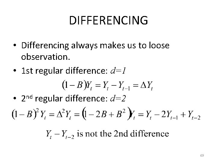
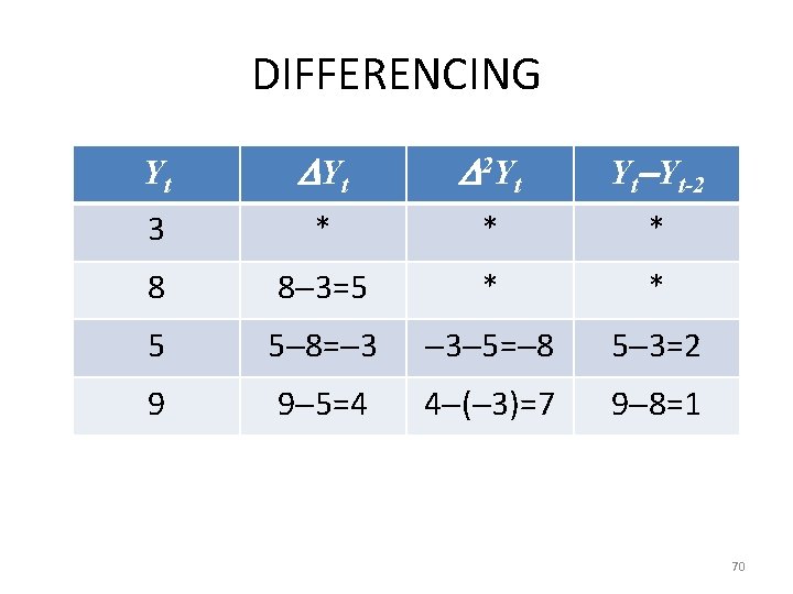
DIFFERENCING • Differencing always makes us to loose observation. • 1 st regular difference: d=1 • 2 nd regular difference: d=2 69

DIFFERENCING Yt 2 Yt Yt Yt-2 3 * * * 8 8 3=5 * * 5 5 8= 3 3 5= 8 5 3=2 9 9 5=4 4 ( 3)=7 9 8=1 70

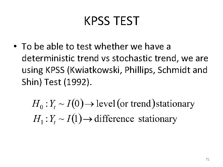
KPSS TEST • To be able to test whether we have a deterministic trend vs stochastic trend, we are using KPSS (Kwiatkowski, Phillips, Schmidt and Shin) Test (1992). 71

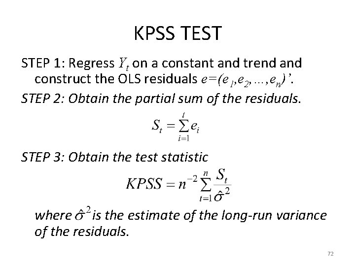
KPSS TEST STEP 1: Regress Yt on a constant and trend and construct the OLS residuals e=(e 1, e 2, …, en)’. STEP 2: Obtain the partial sum of the residuals. STEP 3: Obtain the test statistic where is the estimate of the long-run variance of the residuals. 72

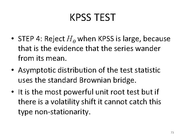
KPSS TEST • STEP 4: Reject H 0 when KPSS is large, because that is the evidence that the series wander from its mean. • Asymptotic distribution of the test statistic uses the standard Brownian bridge. • It is the most powerful unit root test but if there is a volatility shift it cannot catch this type non-stationarity. 73

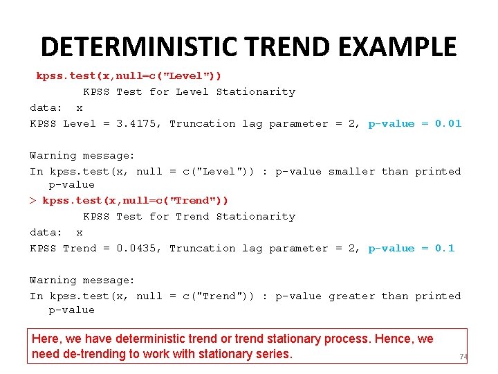
DETERMINISTIC TREND EXAMPLE kpss. test(x, null=c("Level")) KPSS Test for Level Stationarity data: x KPSS Level = 3. 4175, Truncation lag parameter = 2, p-value = 0. 01 Warning message: In kpss. test(x, null = c("Level")) : p-value smaller than printed p-value > kpss. test(x, null=c("Trend")) KPSS Test for Trend Stationarity data: x KPSS Trend = 0. 0435, Truncation lag parameter = 2, p-value = 0. 1 Warning message: In kpss. test(x, null = c("Trend")) : p-value greater than printed p-value Here, we have deterministic trend or trend stationary process. Hence, we need de-trending to work with stationary series. 74

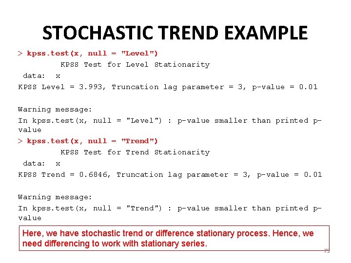
STOCHASTIC TREND EXAMPLE > kpss. test(x, null = "Level") KPSS Test for Level Stationarity data: x KPSS Level = 3. 993, Truncation lag parameter = 3, p-value = 0. 01 Warning message: In kpss. test(x, null = "Level") : p-value smaller than printed pvalue > kpss. test(x, null = "Trend") KPSS Test for Trend Stationarity data: x KPSS Trend = 0. 6846, Truncation lag parameter = 3, p-value = 0. 01 Warning message: In kpss. test(x, null = "Trend") : p-value smaller than printed pvalue Here, we have stochastic trend or difference stationary process. Hence, we need differencing to work with stationary series. 75

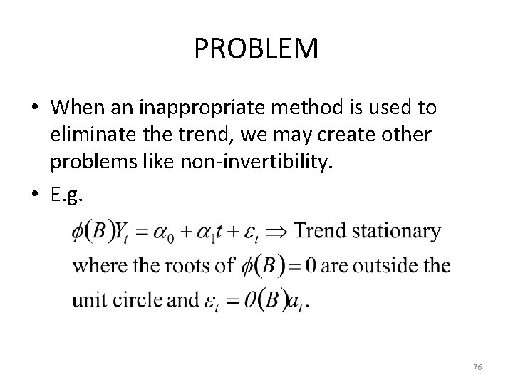
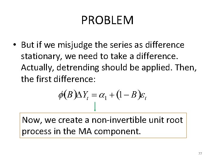
PROBLEM • When an inappropriate method is used to eliminate the trend, we may create other problems like non-invertibility. • E. g. 76

PROBLEM • But if we misjudge the series as difference stationary, we need to take a difference. Actually, detrending should be applied. Then, the first difference: Now, we create a non-invertible unit root process in the MA component. 77

PROBLEM • To overcome this, look at the inverse sample autocorrelation function. If it has the same ACF pattern of non-stationary process (that is, slow decaying behavior), this means that we over-differenced the series. • Go back and de-trend the series instead of differencing. • There also smoothing filters to eliminate the trend (Decomposition Methods). 78

NON-STATIONARITY IN VARIANCE • Stationarity in mean Stationarity in variance • Non-stationarity in mean Non-stationarity in variance • If the mean function is time dependent, 1. The variance, Var(Yt) is time dependent. 2. Var(Yt) is unbounded as t . 3. Autocovariance and autocorrelation functions are also time dependent. 4. If t is large wrt Y 0, then k 1. 79

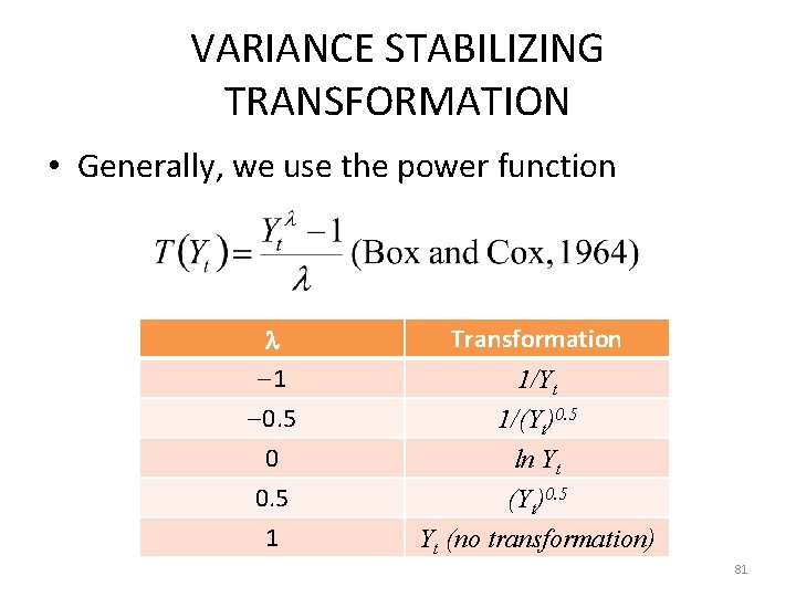
VARIANCE STABILIZING TRANSFORMATION • The variance of a non-stationary process changes as its level changes for some positive constant c and a function f. • Find a function T so that the transformed series T(Yt) has a constant variance. The Delta Method 80

VARIANCE STABILIZING TRANSFORMATION • Generally, we use the power function 1 0. 5 0 Transformation 0. 5 1 (Yt)0. 5 Yt (no transformation) 1/Yt 1/(Yt)0. 5 ln Yt 81

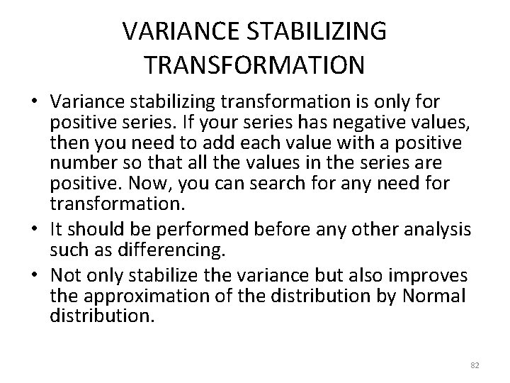
VARIANCE STABILIZING TRANSFORMATION • Variance stabilizing transformation is only for positive series. If your series has negative values, then you need to add each value with a positive number so that all the values in the series are positive. Now, you can search for any need for transformation. • It should be performed before any other analysis such as differencing. • Not only stabilize the variance but also improves the approximation of the distribution by Normal distribution. 82

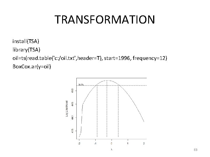
TRANSFORMATION install(TSA) library(TSA) oil=ts(read. table('c: /oil. txt', header=T), start=1996, frequency=12) Box. Cox. ar(y=oil) 83