STAT 497 LECTURE NOTES 9 ESTIMATION 1 ESTIMATION

STAT 497 LECTURE NOTES 9 ESTIMATION 1

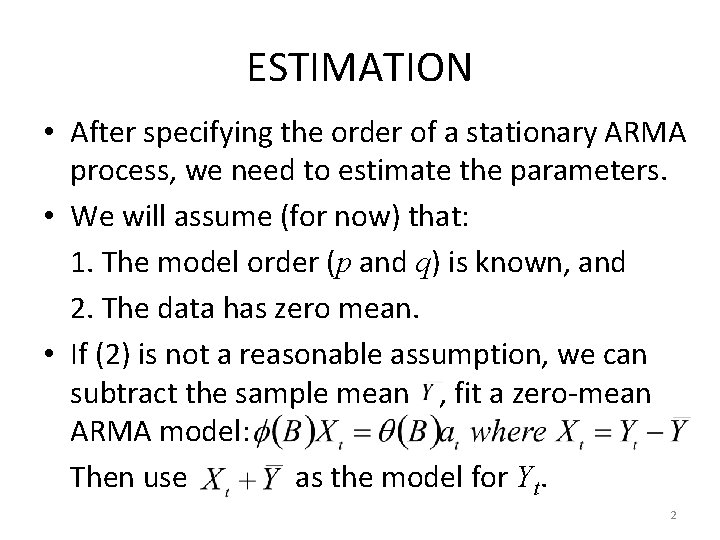
ESTIMATION • After specifying the order of a stationary ARMA process, we need to estimate the parameters. • We will assume (for now) that: 1. The model order (p and q) is known, and 2. The data has zero mean. • If (2) is not a reasonable assumption, we can subtract the sample mean , fit a zero-mean ARMA model: Then use as the model for Yt. 2

ESTIMATION – Method of Moment Estimation (MME) – Ordinary Least Squares (OLS) Estimation – Maximum Likelihood Estimation (MLE) – Least Squares Estimation • Conditional • Unconditional 3

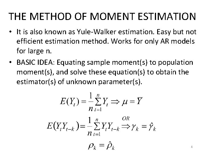
THE METHOD OF MOMENT ESTIMATION • It is also known as Yule-Walker estimation. Easy but not efficient estimation method. Works for only AR models for large n. • BASIC IDEA: Equating sample moment(s) to population moment(s), and solve these equation(s) to obtain the estimator(s) of unknown parameter(s). 4

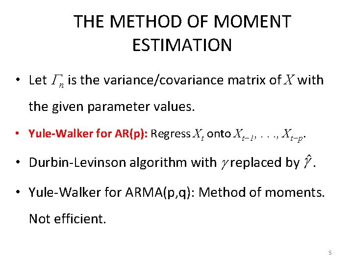
THE METHOD OF MOMENT ESTIMATION • Let n is the variance/covariance matrix of X with the given parameter values. • Yule-Walker for AR(p): Regress Xt onto Xt− 1, . . . , Xt−p. • Durbin-Levinson algorithm with replaced by. • Yule-Walker for ARMA(p, q): Method of moments. Not efficient. 5

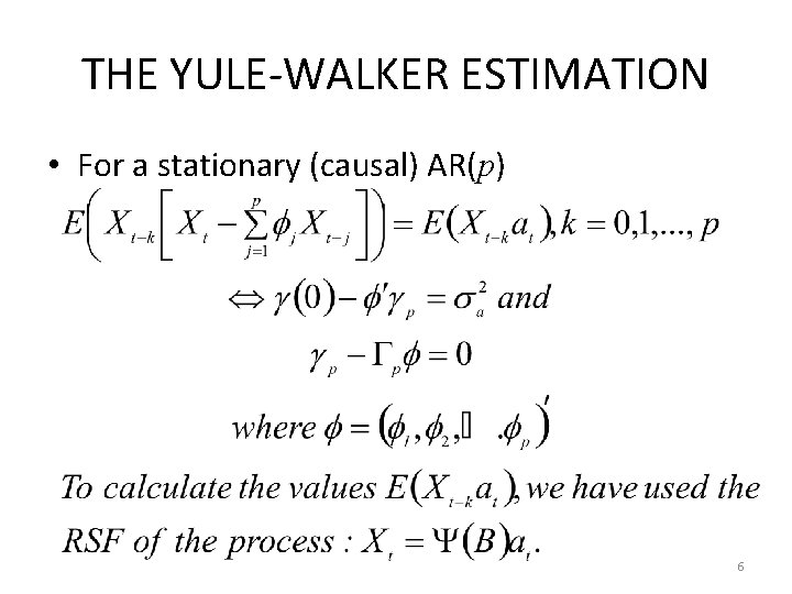
THE YULE-WALKER ESTIMATION • For a stationary (causal) AR(p) 6

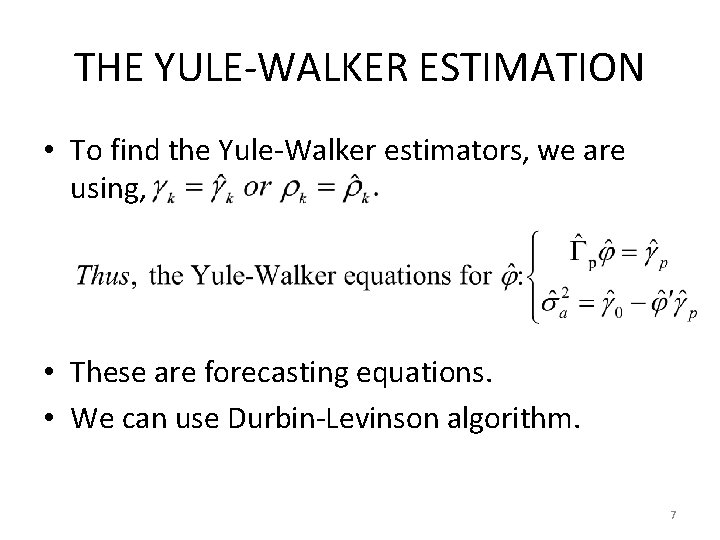
THE YULE-WALKER ESTIMATION • To find the Yule-Walker estimators, we are using, • These are forecasting equations. • We can use Durbin-Levinson algorithm. 7

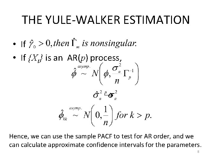
THE YULE-WALKER ESTIMATION • If {Xt} is an AR(p) process, Hence, we can use the sample PACF to test for AR order, and we can calculate approximate confidence intervals for the parameters. 8

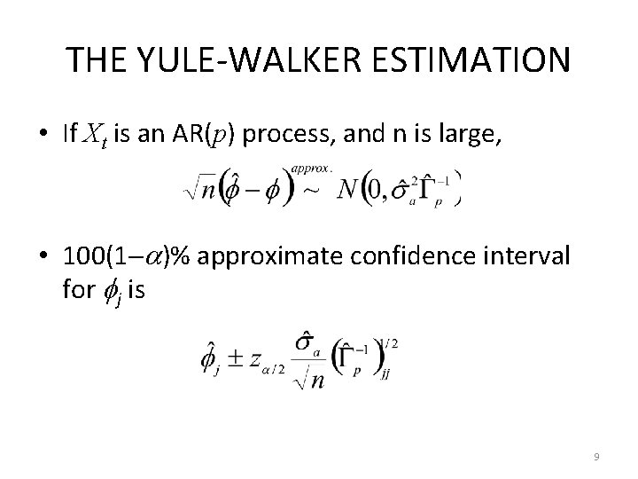
THE YULE-WALKER ESTIMATION • If Xt is an AR(p) process, and n is large, • 100(1 )% approximate confidence interval for j is 9

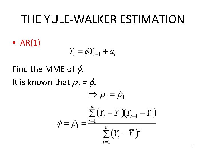
THE YULE-WALKER ESTIMATION • AR(1) Find the MME of . It is known that 1 = . 10

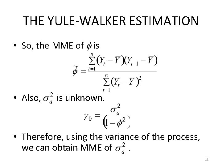
THE YULE-WALKER ESTIMATION • So, the MME of is • Also, is unknown. • Therefore, using the variance of the process, we can obtain MME of. 11

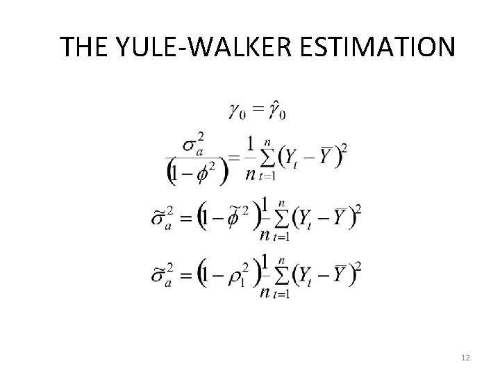
THE YULE-WALKER ESTIMATION 12

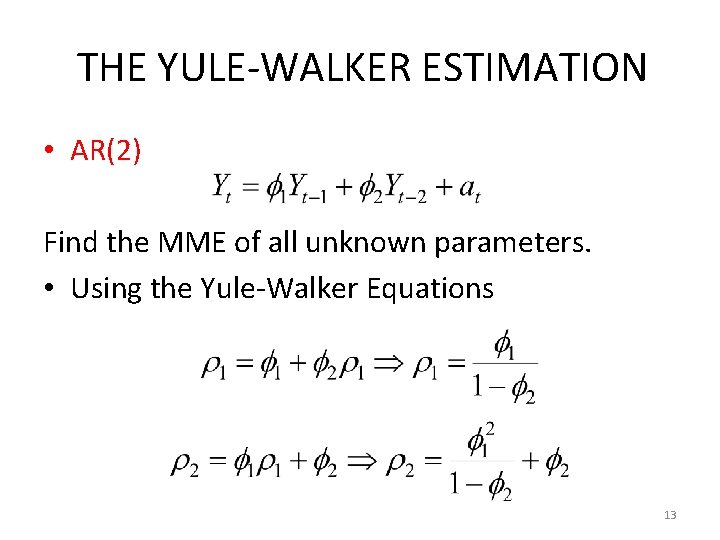
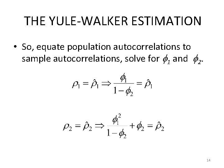
THE YULE-WALKER ESTIMATION • AR(2) Find the MME of all unknown parameters. • Using the Yule-Walker Equations 13

THE YULE-WALKER ESTIMATION • So, equate population autocorrelations to sample autocorrelations, solve for 1 and 2. 14

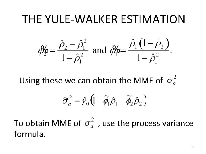
THE YULE-WALKER ESTIMATION Using these we can obtain the MME of To obtain MME of formula. , use the process variance 15

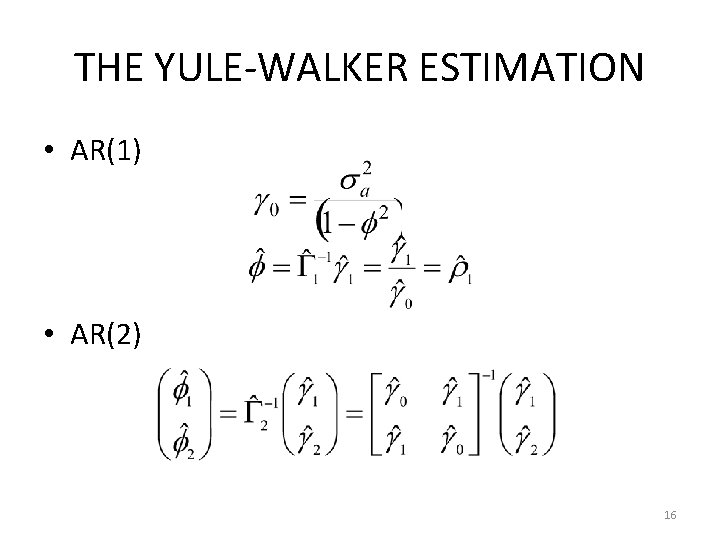
THE YULE-WALKER ESTIMATION • AR(1) • AR(2) 16

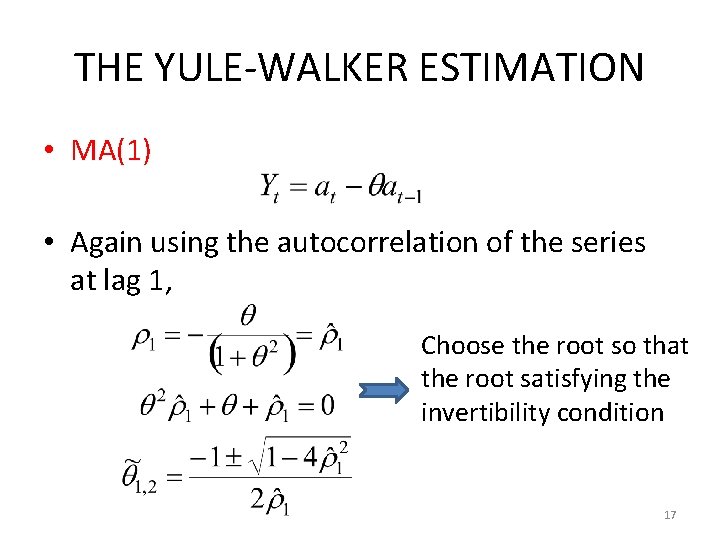
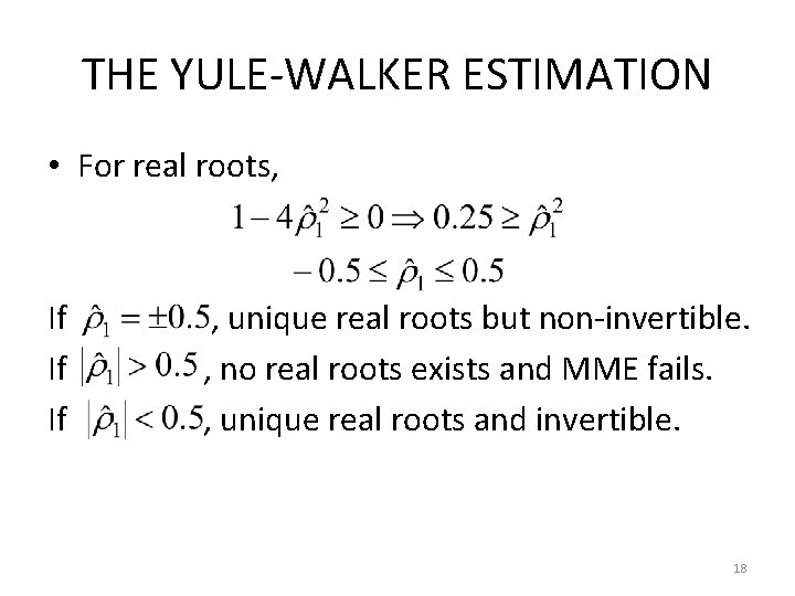
THE YULE-WALKER ESTIMATION • MA(1) • Again using the autocorrelation of the series at lag 1, Choose the root so that the root satisfying the invertibility condition 17

THE YULE-WALKER ESTIMATION • For real roots, If If If , unique real roots but non-invertible. , no real roots exists and MME fails. , unique real roots and invertible. 18

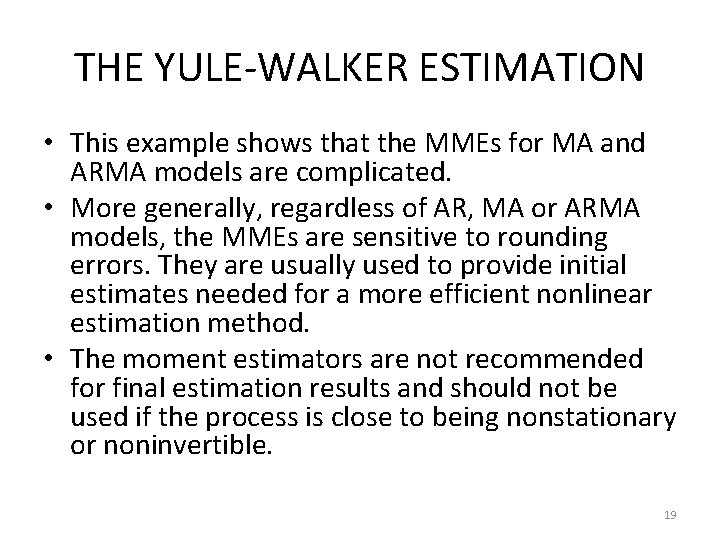
THE YULE-WALKER ESTIMATION • This example shows that the MMEs for MA and ARMA models are complicated. • More generally, regardless of AR, MA or ARMA models, the MMEs are sensitive to rounding errors. They are usually used to provide initial estimates needed for a more efficient nonlinear estimation method. • The moment estimators are not recommended for final estimation results and should not be used if the process is close to being nonstationary or noninvertible. 19

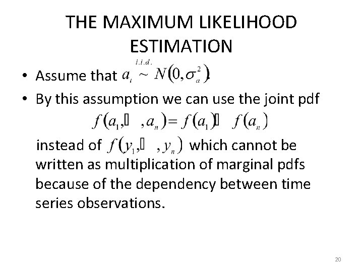
THE MAXIMUM LIKELIHOOD ESTIMATION • Assume that • By this assumption we can use the joint pdf instead of which cannot be written as multiplication of marginal pdfs because of the dependency between time series observations. 20

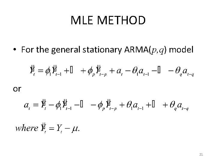
MLE METHOD • For the general stationary ARMA(p, q) model or 21

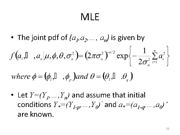
MLE • The joint pdf of (a 1, a 2, …, an) is given by • Let Y=(Y 1, …, Yn) and assume that initial conditions Y*=(Y 1 -p, …, Y 0)’ and a*=(a 1 -q, …, a 0)’ are known. 22

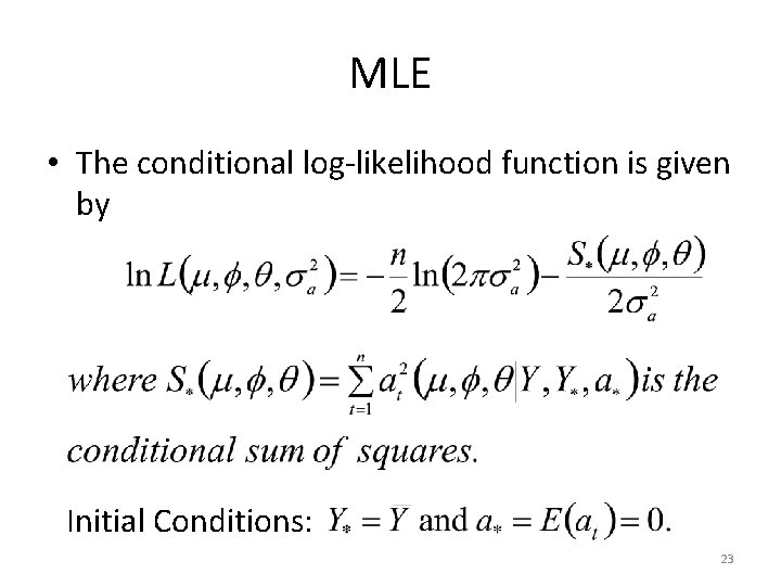
MLE • The conditional log-likelihood function is given by Initial Conditions: 23

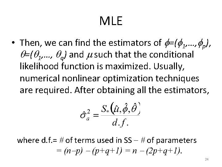
MLE • Then, we can find the estimators of =( 1, …, p), =( 1, …, q) and such that the conditional likelihood function is maximized. Usually, numerical nonlinear optimization techniques are required. After obtaining all the estimators, where d. f. = of terms used in SS of parameters = (n p) (p+q+1) = n (2 p+q+1). 24

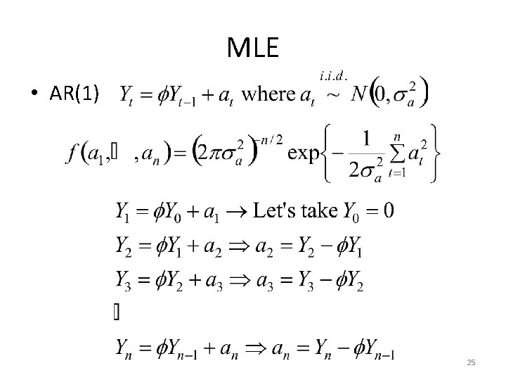
MLE • AR(1) 25

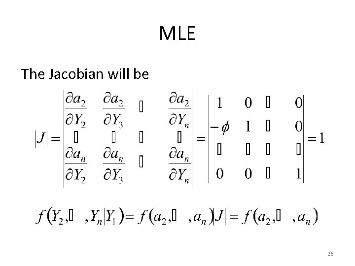
MLE The Jacobian will be 26

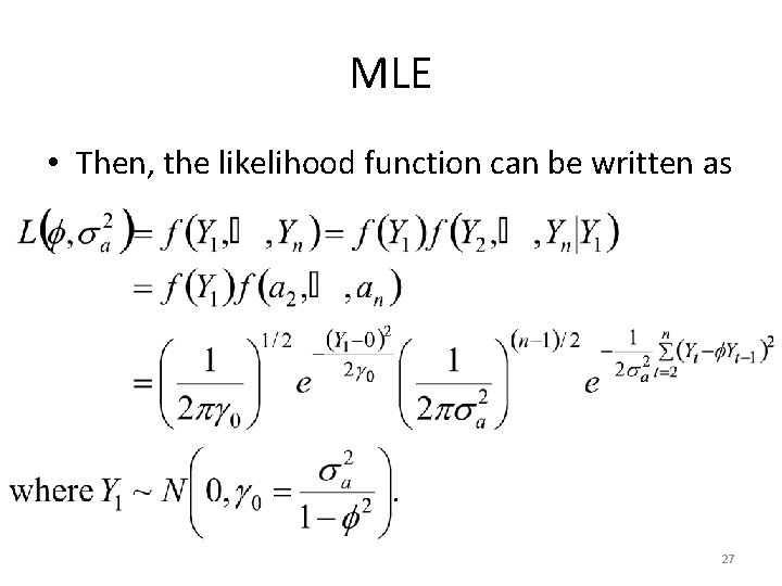
MLE • Then, the likelihood function can be written as 27

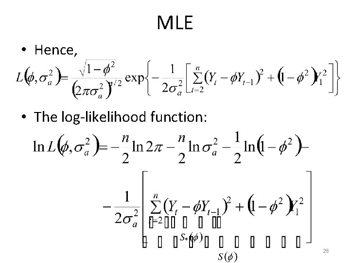
MLE • Hence, • The log-likelihood function: 28

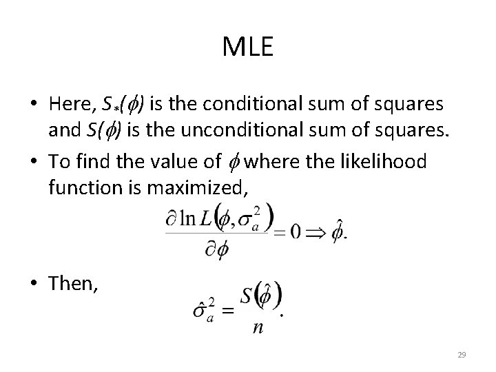
MLE • Here, S*( ) is the conditional sum of squares and S( ) is the unconditional sum of squares. • To find the value of where the likelihood function is maximized, • Then, 29

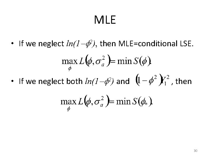
MLE • If we neglect ln(1 2), then MLE=conditional LSE. • If we neglect both ln(1 2) and , then 30

MLE • Asymptotically unbiased, efficient, consistent, sufficient for large sample sizes but hard to deal with joint pdf. 31

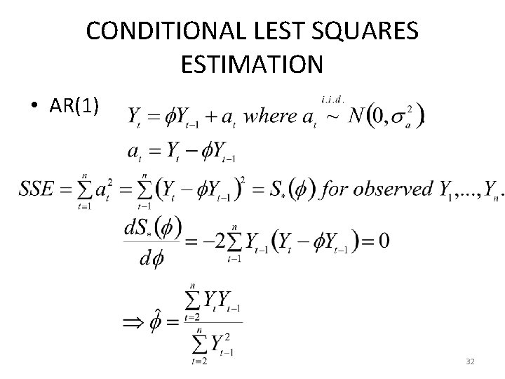
CONDITIONAL LEST SQUARES ESTIMATION • AR(1) 32

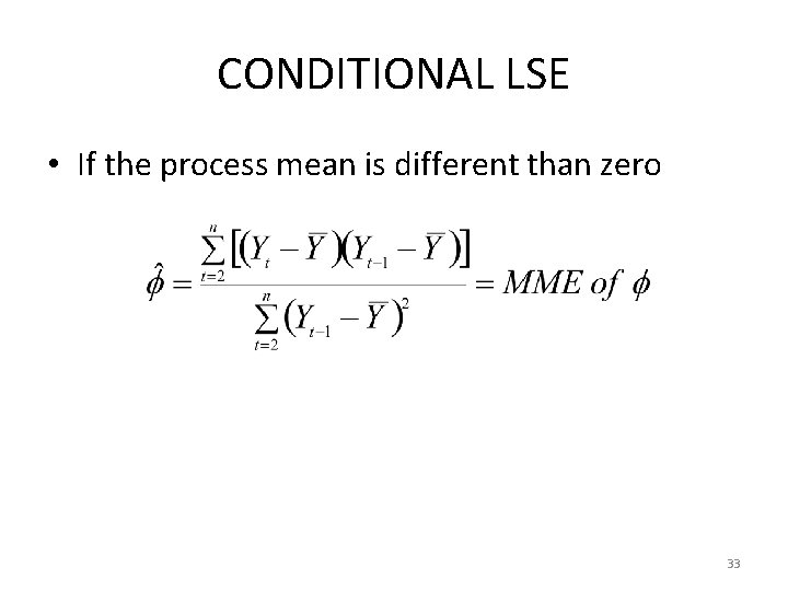
CONDITIONAL LSE • If the process mean is different than zero 33

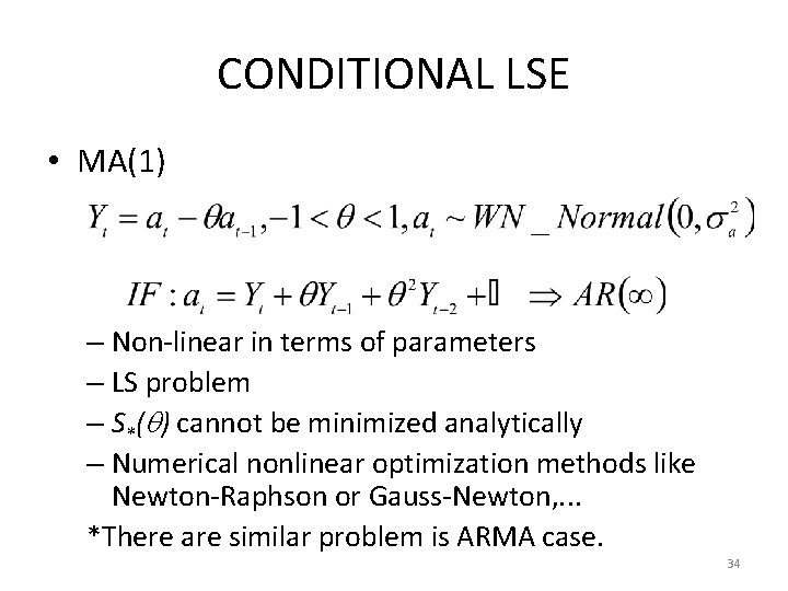
CONDITIONAL LSE • MA(1) – Non-linear in terms of parameters – LS problem – S*( ) cannot be minimized analytically – Numerical nonlinear optimization methods like Newton-Raphson or Gauss-Newton, . . . *There are similar problem is ARMA case. 34

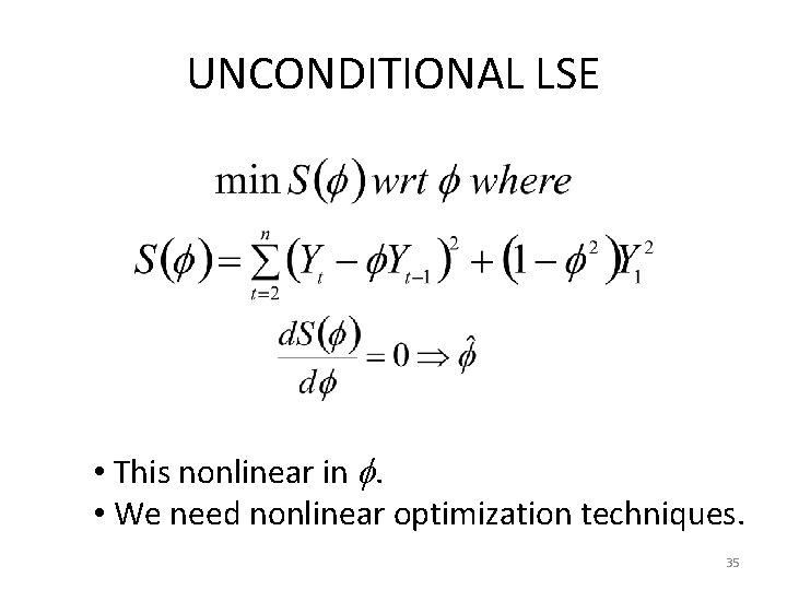
UNCONDITIONAL LSE • This nonlinear in . • We need nonlinear optimization techniques. 35

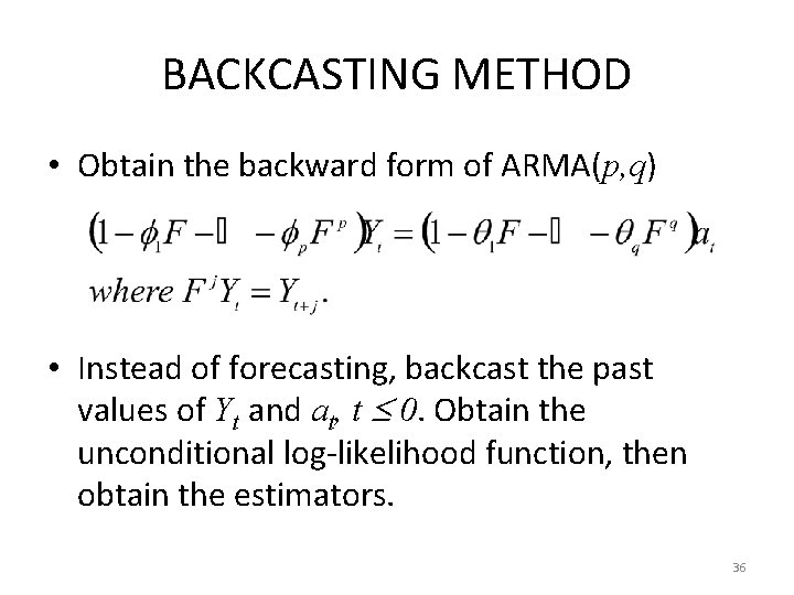
BACKCASTING METHOD • Obtain the backward form of ARMA(p, q) • Instead of forecasting, backcast the past values of Yt and at, t 0. Obtain the unconditional log-likelihood function, then obtain the estimators. 36

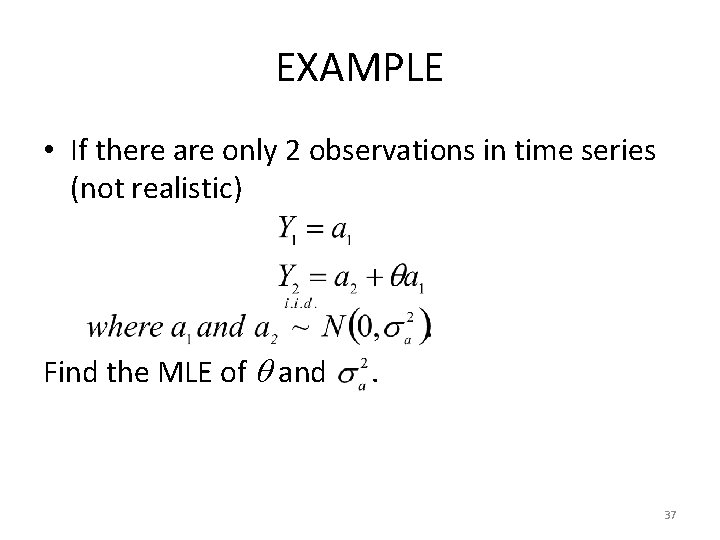
EXAMPLE • If there are only 2 observations in time series (not realistic) Find the MLE of and . 37

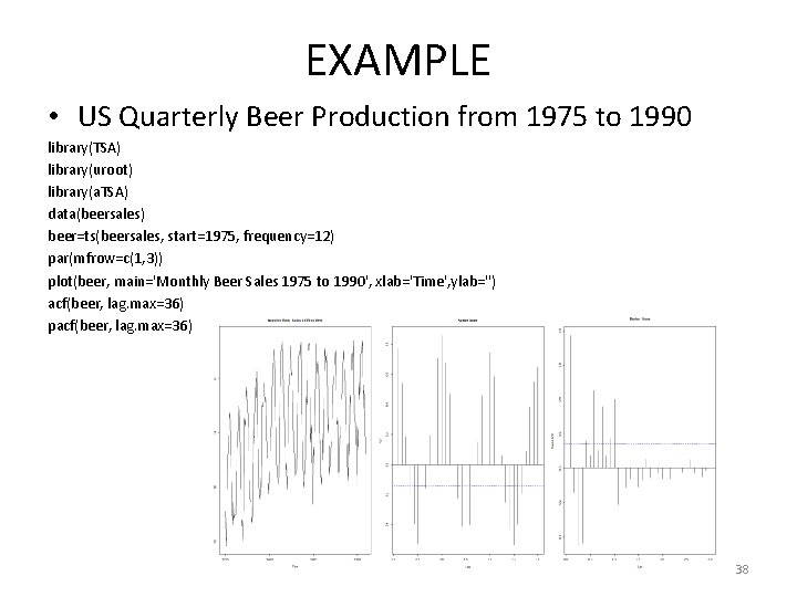
EXAMPLE • US Quarterly Beer Production from 1975 to 1990 library(TSA) library(uroot) library(a. TSA) data(beersales) beer=ts(beersales, start=1975, frequency=12) par(mfrow=c(1, 3)) plot(beer, main='Monthly Beer Sales 1975 to 1990', xlab='Time', ylab='') acf(beer, lag. max=36) pacf(beer, lag. max=36) 38

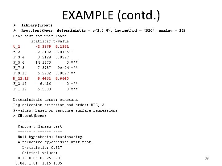
EXAMPLE (contd. ) Ø library(uroot) Ø hegy. test(beer, deterministic = c(1, 0, 0), lag. method = "BIC", maxlag = 12) HEGY test for unit roots statistic p-value t_1 -2. 2779 0. 1281 t_2 -2. 2102 0. 0185 * F_3: 4 0. 2129 0. 8227 F_5: 6 14. 1673 0 *** F_7: 8 7. 3787 9 e-04 *** F_9: 10 6. 2202 0. 0027 ** F_11: 12 0. 4434 0. 6645 F_2: 12 6. 416 0 *** F_1: 12 6. 3383 0 *** Deterministic terms: constant Lag selection criterion and order: BIC, 2 P-values: based on response surface regressions > CH. test(beer) ------ ---Canova & Hansen test ------ ---Null hypothesis: Stationarity. Alternative hypothesis: Unit root. L-statistic: 0. 817 Critical values: 0. 10 0. 05 0. 025 0. 01 0. 846 1. 01 1. 16 1. 35 39

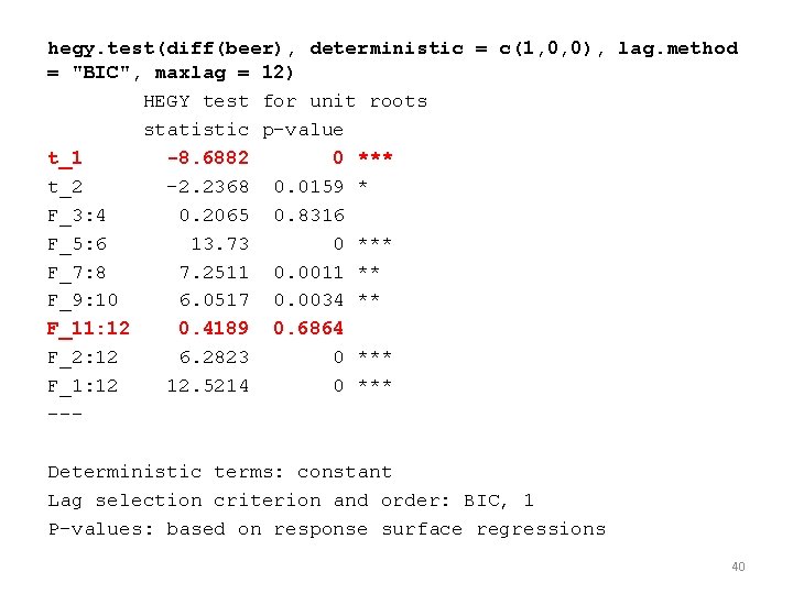
hegy. test(diff(beer), deterministic = c(1, 0, 0), lag. method = "BIC", maxlag = 12) HEGY test for unit roots statistic p-value t_1 -8. 6882 0 *** t_2 -2. 2368 0. 0159 * F_3: 4 0. 2065 0. 8316 F_5: 6 13. 73 0 *** F_7: 8 7. 2511 0. 0011 ** F_9: 10 6. 0517 0. 0034 ** F_11: 12 0. 4189 0. 6864 F_2: 12 6. 2823 0 *** F_1: 12 12. 5214 0 *** --Deterministic terms: constant Lag selection criterion and order: BIC, 1 P-values: based on response surface regressions 40

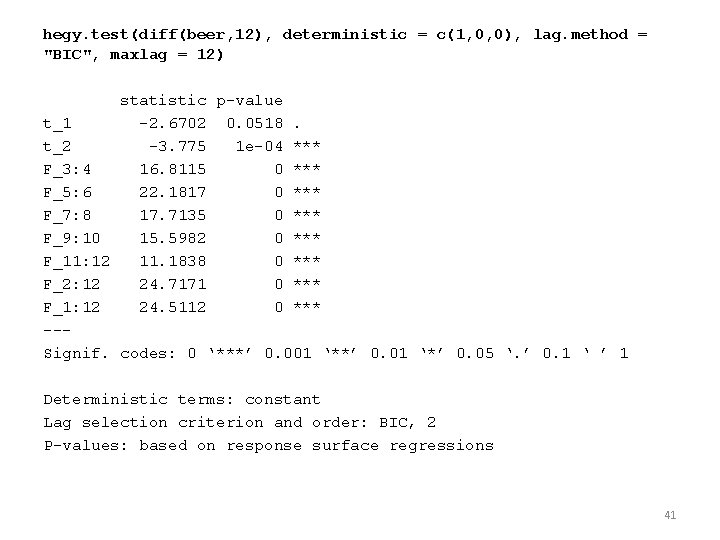
hegy. test(diff(beer, 12), deterministic = c(1, 0, 0), lag. method = "BIC", maxlag = 12) statistic p-value t_1 -2. 6702 0. 0518. t_2 -3. 775 1 e-04 *** F_3: 4 16. 8115 0 *** F_5: 6 22. 1817 0 *** F_7: 8 17. 7135 0 *** F_9: 10 15. 5982 0 *** F_11: 12 11. 1838 0 *** F_2: 12 24. 7171 0 *** F_1: 12 24. 5112 0 *** --Signif. codes: 0 ‘***’ 0. 001 ‘**’ 0. 01 ‘*’ 0. 05 ‘. ’ 0. 1 ‘ ’ 1 Deterministic terms: constant Lag selection criterion and order: BIC, 2 P-values: based on response surface regressions 41

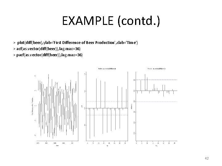
EXAMPLE (contd. ) > plot(diff(beer), ylab='First Difference of Beer Production', xlab='Time') > acf(as. vector(diff(beer)), lag. max=36) > pacf(as. vector(diff(beer)), lag. max=36) 42

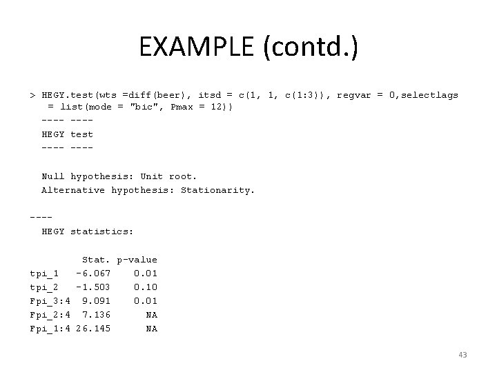
EXAMPLE (contd. ) > HEGY. test(wts =diff(beer), itsd = c(1, 1, c(1: 3)), regvar = 0, selectlags = list(mode = "bic", Pmax = 12)) ---- ---HEGY test ---- ---Null hypothesis: Unit root. Alternative hypothesis: Stationarity. ---HEGY statistics: Stat. p-value tpi_1 -6. 067 0. 01 tpi_2 -1. 503 0. 10 Fpi_3: 4 9. 091 0. 01 Fpi_2: 4 7. 136 NA Fpi_1: 4 26. 145 NA 43

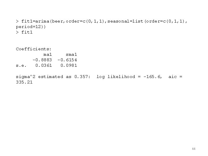
> fit 1=arima(beer, order=c(0, 1, 1), seasonal=list(order=c(0, 1, 1), period=12)) > fit 1 Coefficients: ma 1 -0. 8883 s. e. 0. 0361 sma 1 -0. 6154 0. 0981 sigma^2 estimated as 0. 357: 335. 21 log likelihood = -165. 6, aic = 44

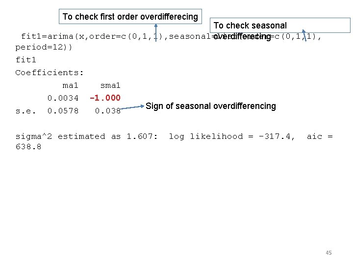
To check first order overdifferecing To check seasonal fit 1=arima(x, order=c(0, 1, 1), seasonal=list(order=c(0, 1, 1), overdifferecing period=12)) fit 1 Coefficients: ma 1 sma 1 0. 0034 -1. 000 Sign of seasonal overdifferencing s. e. 0. 0578 0. 038 sigma^2 estimated as 1. 607: 638. 8 log likelihood = -317. 4, aic = 45

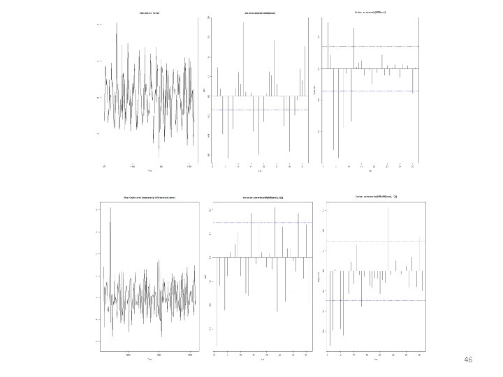
46

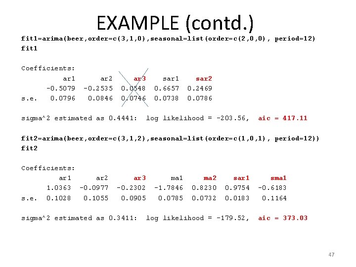
EXAMPLE (contd. ) fit 1=arima(beer, order=c(3, 1, 0), seasonal=list(order=c(2, 0, 0), period=12) fit 1 Coefficients: ar 1 -0. 5079 s. e. 0. 0796 ar 2 -0. 2535 0. 0846 ar 3 0. 0548 0. 0746 sigma^2 estimated as 0. 4441: sar 1 0. 6657 0. 0738 sar 2 0. 2469 0. 0786 log likelihood = -203. 56, aic = 417. 11 fit 2=arima(beer, order=c(3, 1, 2), seasonal=list(order=c(1, 0, 1), period=12)) fit 2 Coefficients: ar 1 ar 2 1. 0363 -0. 0977 s. e. 0. 1028 0. 1055 ar 3 -0. 2302 0. 0905 sigma^2 estimated as 0. 3411: ma 1 -1. 7846 0. 0785 ma 2 0. 8230 0. 0732 sar 1 0. 9754 0. 0183 log likelihood = -179. 52, sma 1 -0. 6183 0. 1164 aic = 373. 03 47

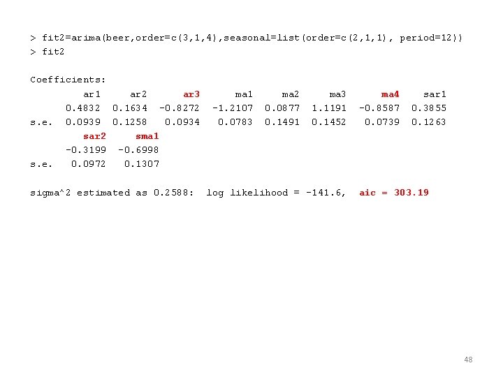
> fit 2=arima(beer, order=c(3, 1, 4), seasonal=list(order=c(2, 1, 1), period=12)) > fit 2 Coefficients: ar 1 ar 2 ar 3 0. 4832 0. 1634 -0. 8272 s. e. 0. 0939 0. 1258 0. 0934 sar 2 sma 1 -0. 3199 -0. 6998 s. e. 0. 0972 0. 1307 sigma^2 estimated as 0. 2588: ma 1 -1. 2107 0. 0783 ma 2 0. 0877 0. 1491 ma 3 1. 1191 0. 1452 log likelihood = -141. 6, ma 4 -0. 8587 0. 0739 sar 1 0. 3855 0. 1263 aic = 303. 19 48

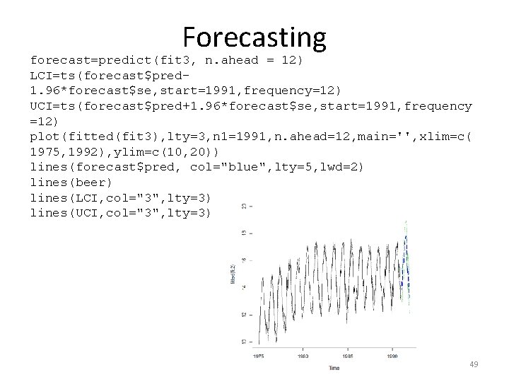
Forecasting forecast=predict(fit 3, n. ahead = 12) LCI=ts(forecast$pred 1. 96*forecast$se, start=1991, frequency=12) UCI=ts(forecast$pred+1. 96*forecast$se, start=1991, frequency =12) plot(fitted(fit 3), lty=3, n 1=1991, n. ahead=12, main='', xlim=c( 1975, 1992), ylim=c(10, 20)) lines(forecast$pred, col="blue", lty=5, lwd=2) lines(beer) lines(LCI, col="3", lty=3) lines(UCI, col="3", lty=3) 49

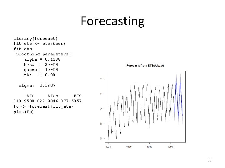
Forecasting library(forecast) fit_ets <- ets(beer) fit_ets Smoothing parameters: alpha = 0. 1138 beta = 2 e-04 gamma = 1 e-04 phi = 0. 98 sigma: 0. 5807 AICc BIC 818. 9508 822. 9046 877. 5857 fc <- forecast(fit_ets) plot(fc) 50

Accuracy Comparison MSE_arima=sum(fit 3$res)^2/length(beer) MSE_ets=sum(fit_ets$res)^2/length(beer) print(cbind(MSE_arima, MSE_ets)) MSE_arima MSE_ets [1, ] 0. 03324427 0. 1303638 51