STAT 497 LECTURE NOTE 13 VAR MODELS AND

STAT 497 LECTURE NOTE 13 VAR MODELS AND GRANGER CAUSALITY 1

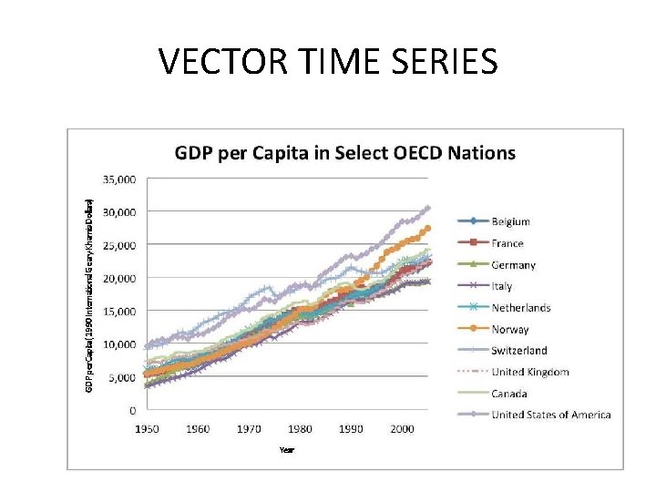
VECTOR TIME SERIES • A vector series consists of multiple single series. • Why we need multiple series? – To be able to understand the relationship between several components – To be able to get better forecasts 2

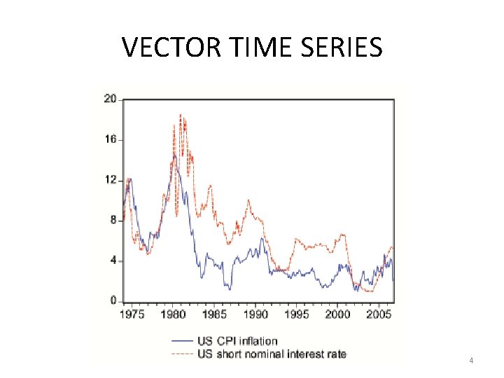
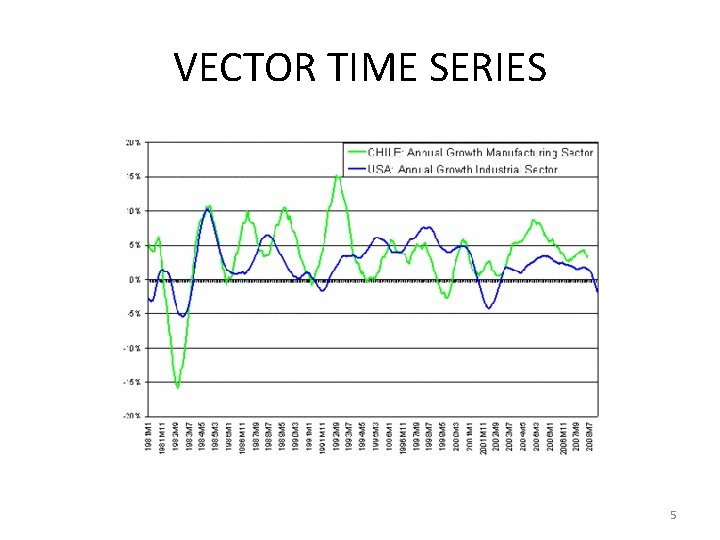
VECTOR TIME SERIES • Price movements in one market can spread easily and instantly to another market. For this reason, financial markets are more dependent on each other than ever before. So, we have to consider them jointly to better understand the dynamic structure of global market. Knowing how markets are interrelated is of great importance in finance. • For an investor or a financial institution holding multiple assets play an important role in decision making. 3

VECTOR TIME SERIES 4

VECTOR TIME SERIES 5

VECTOR TIME SERIES 6

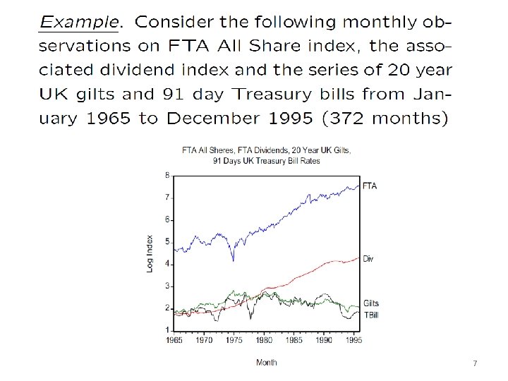
7

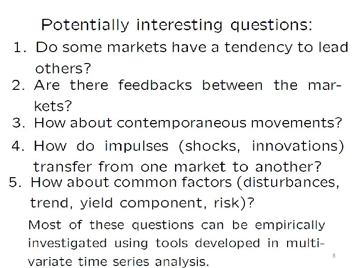
8

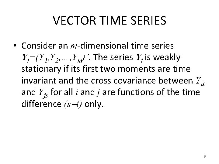
VECTOR TIME SERIES • Consider an m-dimensional time series Yt=(Y 1, Y 2, …, Ym)’. The series Yt is weakly stationary if its first two moments are time invariant and the cross covariance between Yit and Yjs for all i and j are functions of the time difference (s t) only. 9

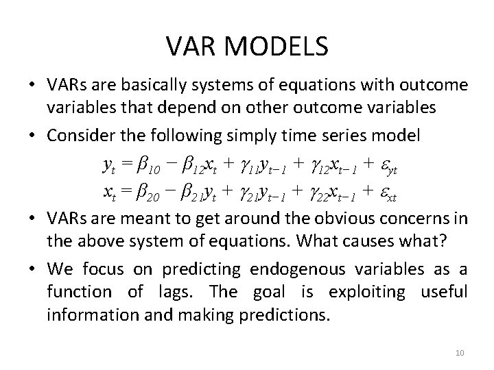
VAR MODELS • VARs are basically systems of equations with outcome variables that depend on other outcome variables • Consider the following simply time series model yt = β 10 − β 12 xt + 11 yt− 1 + 12 xt− 1 + yt xt = β 20 − β 21 yt + 21 yt− 1 + 22 xt− 1 + xt • VARs are meant to get around the obvious concerns in the above system of equations. What causes what? • We focus on predicting endogenous variables as a function of lags. The goal is exploiting useful information and making predictions. 10

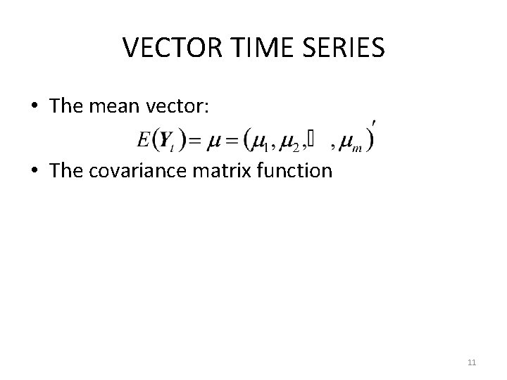
VECTOR TIME SERIES • The mean vector: • The covariance matrix function 11

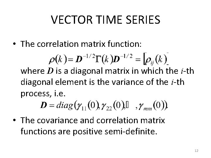
VECTOR TIME SERIES • The correlation matrix function: where D is a diagonal matrix in which the i-th diagonal element is the variance of the i-th process, i. e. • The covariance and correlation matrix functions are positive semi-definite. 12

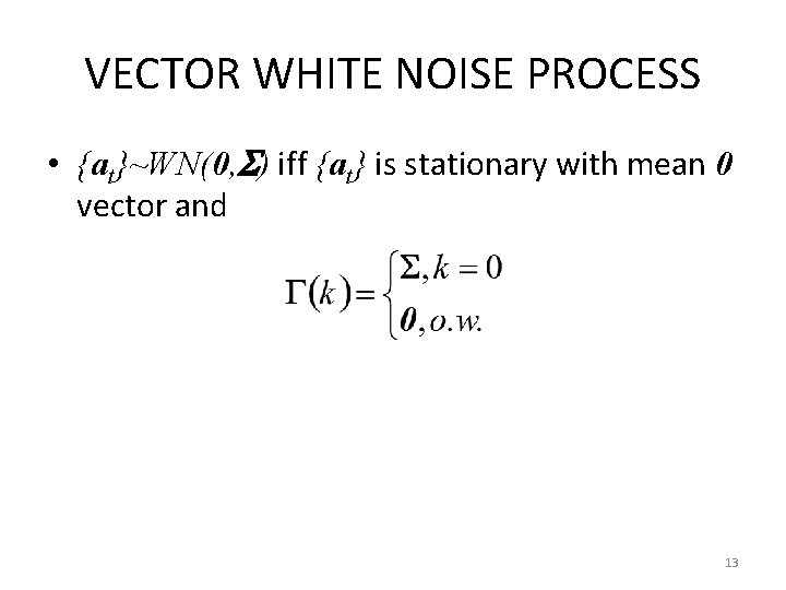
VECTOR WHITE NOISE PROCESS • {at}~WN(0, ) iff {at} is stationary with mean 0 vector and 13

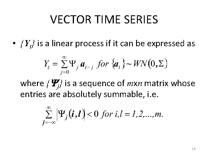
VECTOR TIME SERIES • {Yt} is a linear process if it can be expressed as where { j} is a sequence of mxn matrix whose entries are absolutely summable, i. e. 14

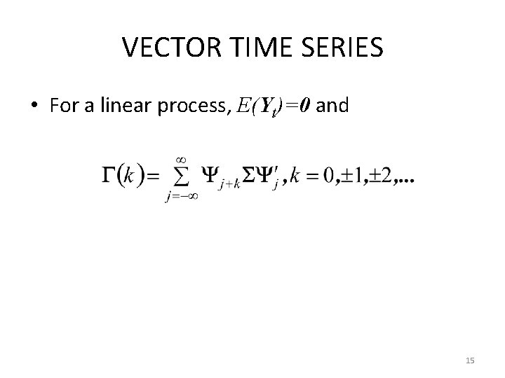
VECTOR TIME SERIES • For a linear process, E(Yt)=0 and 15

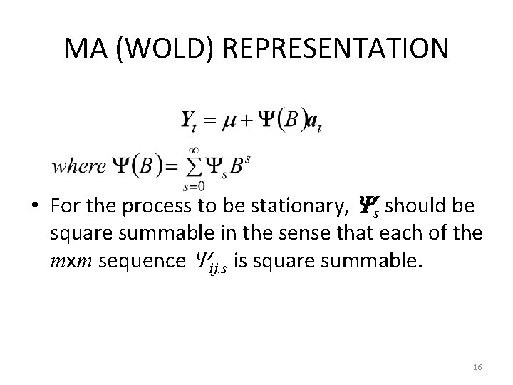
MA (WOLD) REPRESENTATION • For the process to be stationary, s should be square summable in the sense that each of the mxm sequence ij. s is square summable. 16

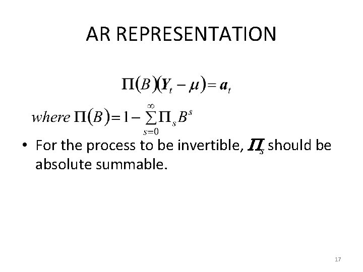
AR REPRESENTATION • For the process to be invertible, s should be absolute summable. 17

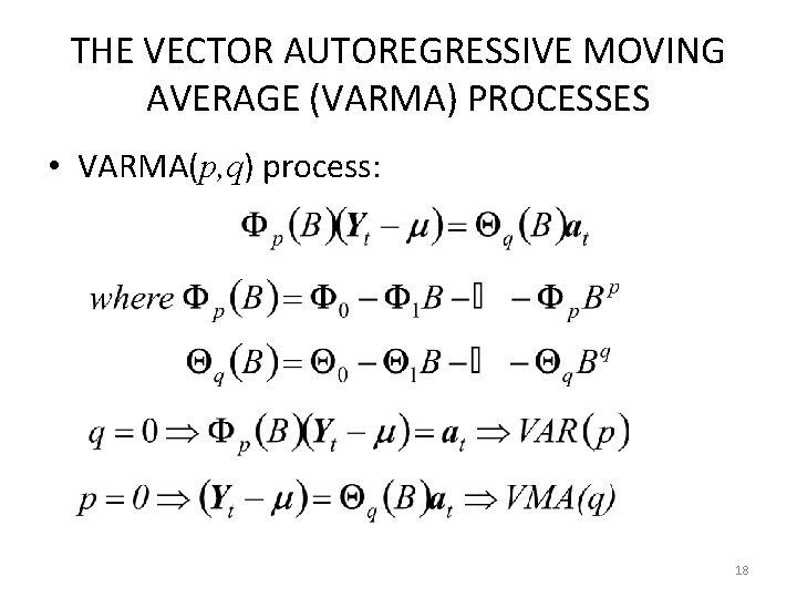
THE VECTOR AUTOREGRESSIVE MOVING AVERAGE (VARMA) PROCESSES • VARMA(p, q) process: 18

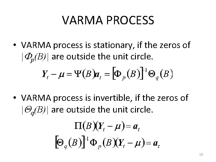
VARMA PROCESS • VARMA process is stationary, if the zeros of | p(B)| are outside the unit circle. • VARMA process is invertible, if the zeros of | q(B)| are outside the unit circle. 19

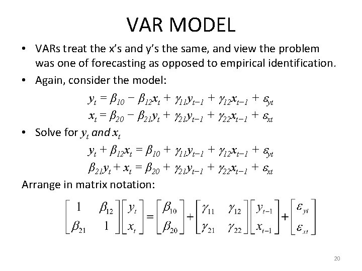
VAR MODEL • VARs treat the x’s and y’s the same, and view the problem was one of forecasting as opposed to empirical identification. • Again, consider the model: yt = β 10 − β 12 xt + 11 yt− 1 + 12 xt− 1 + yt xt = β 20 − β 21 yt + 21 yt− 1 + 22 xt− 1 + xt • Solve for yt and xt yt + β 12 xt = β 10 + 11 yt− 1 + 12 xt− 1 + yt β 21 yt + xt = β 20 + 21 yt− 1 + 22 xt− 1 + xt Arrange in matrix notation: 20

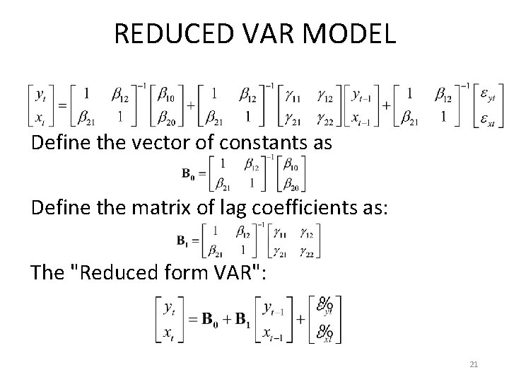
REDUCED VAR MODEL Define the vector of constants as Define the matrix of lag coefficients as: The "Reduced form VAR": 21

IDENTIFIBILITY PROBLEM • Multiplying matrices by some arbitrary matrix polynomial may give us an identical covariance matrix. So, the VARMA(p, q) model is not identifiable. We cannot uniquely determine p and q. 22

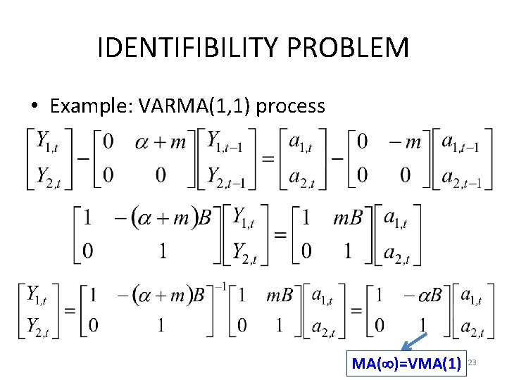
IDENTIFIBILITY PROBLEM • Example: VARMA(1, 1) process MA( )=VMA(1) 23

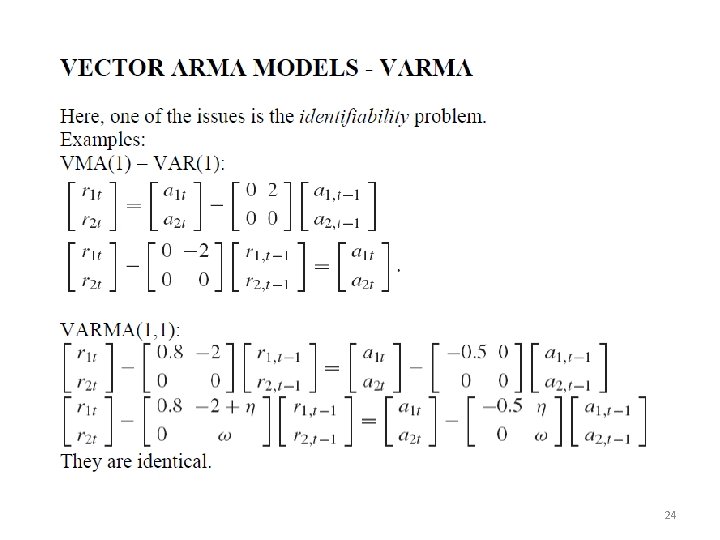
24

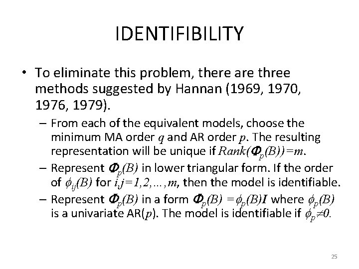
IDENTIFIBILITY • To eliminate this problem, there are three methods suggested by Hannan (1969, 1970, 1976, 1979). – From each of the equivalent models, choose the minimum MA order q and AR order p. The resulting representation will be unique if Rank( p(B))=m. – Represent p(B) in lower triangular form. If the order of ij(B) for i, j=1, 2, …, m, then the model is identifiable. – Represent p(B) in a form p(B) = p(B)I where p(B) is a univariate AR(p). The model is identifiable if p 0. 25

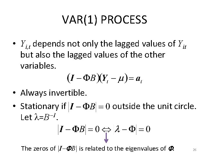
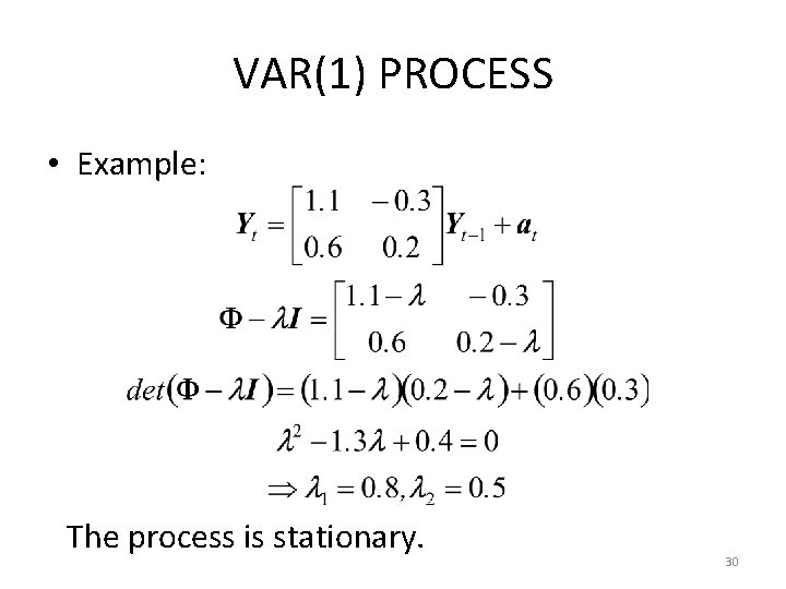
VAR(1) PROCESS • Yi, t depends not only the lagged values of Yit but also the lagged values of the other variables. • Always invertible. • Stationary if Let =B 1. outside the unit circle. The zeros of |I B| is related to the eigenvalues of . 26

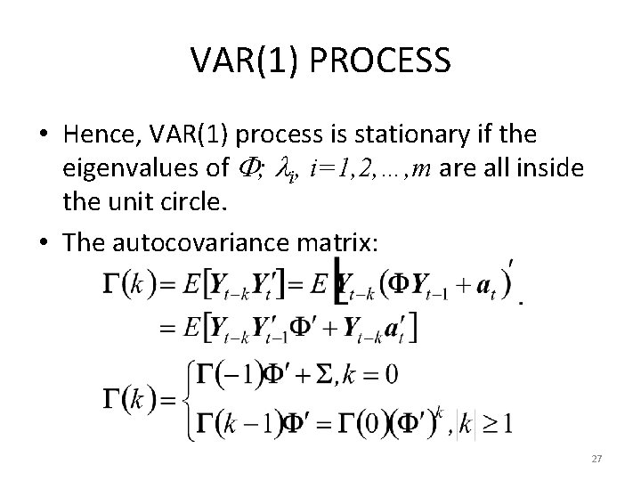
VAR(1) PROCESS • Hence, VAR(1) process is stationary if the eigenvalues of ; i, i=1, 2, …, m are all inside the unit circle. • The autocovariance matrix: 27

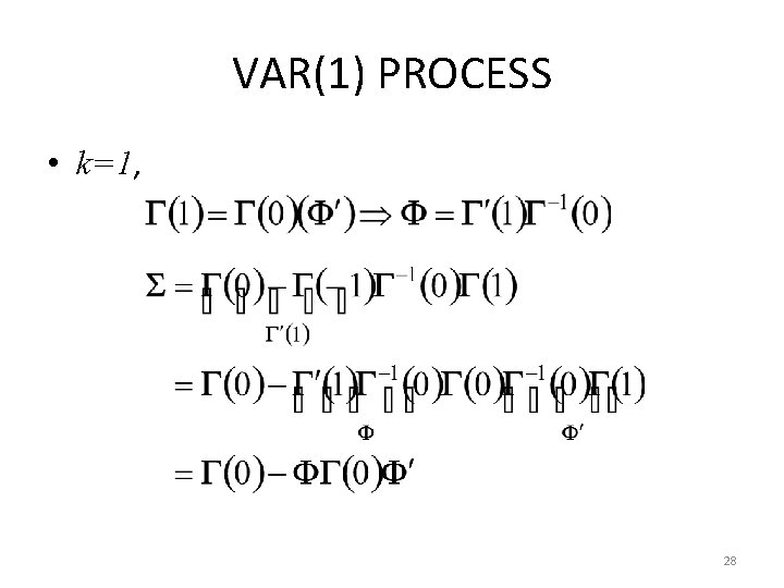
VAR(1) PROCESS • k=1, 28

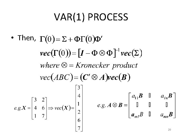
VAR(1) PROCESS • Then, 29

VAR(1) PROCESS • Example: The process is stationary. 30

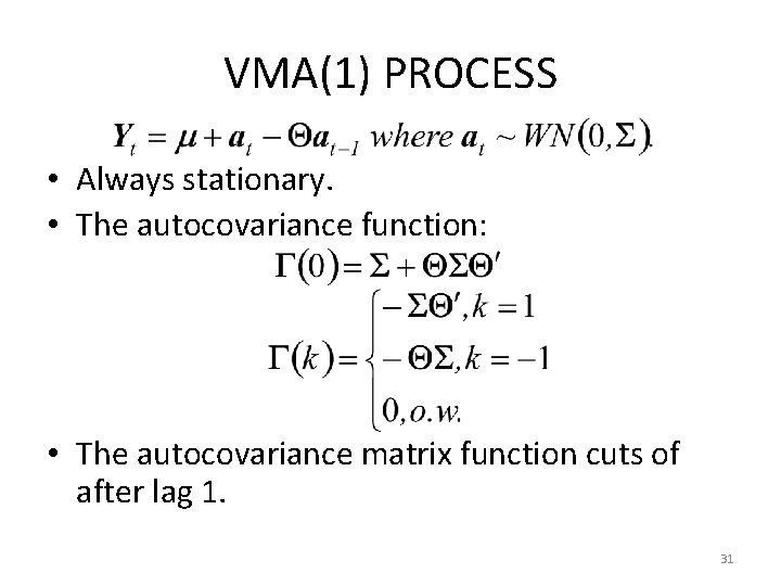
VMA(1) PROCESS • Always stationary. • The autocovariance function: • The autocovariance matrix function cuts of after lag 1. 31

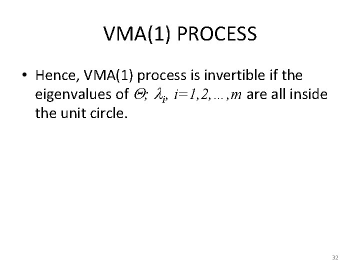
VMA(1) PROCESS • Hence, VMA(1) process is invertible if the eigenvalues of ; i, i=1, 2, …, m are all inside the unit circle. 32

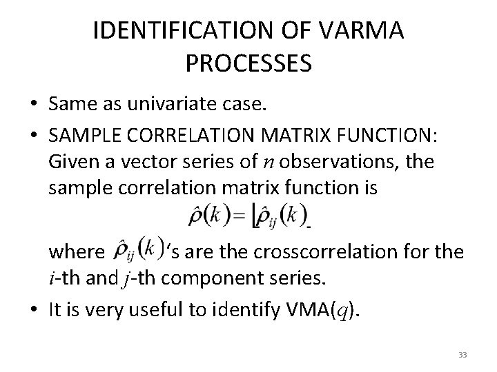
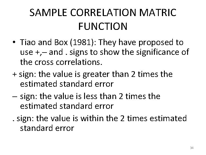
IDENTIFICATION OF VARMA PROCESSES • Same as univariate case. • SAMPLE CORRELATION MATRIX FUNCTION: Given a vector series of n observations, the sample correlation matrix function is where ‘s are the crosscorrelation for the i-th and j-th component series. • It is very useful to identify VMA(q). 33

SAMPLE CORRELATION MATRIC FUNCTION • Tiao and Box (1981): They have proposed to use +, and. signs to show the significance of the cross correlations. + sign: the value is greater than 2 times the estimated standard error sign: the value is less than 2 times the estimated standard error. sign: the value is within the 2 times estimated standard error 34

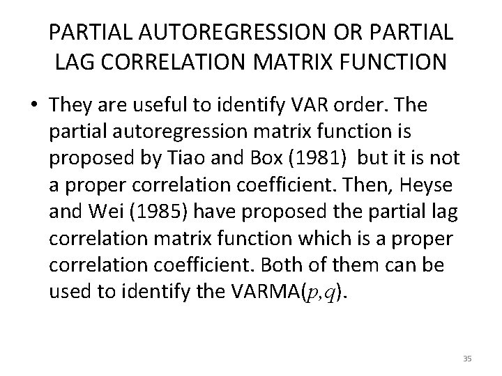
PARTIAL AUTOREGRESSION OR PARTIAL LAG CORRELATION MATRIX FUNCTION • They are useful to identify VAR order. The partial autoregression matrix function is proposed by Tiao and Box (1981) but it is not a proper correlation coefficient. Then, Heyse and Wei (1985) have proposed the partial lag correlation matrix function which is a proper correlation coefficient. Both of them can be used to identify the VARMA(p, q). 35

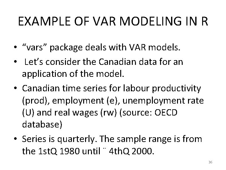
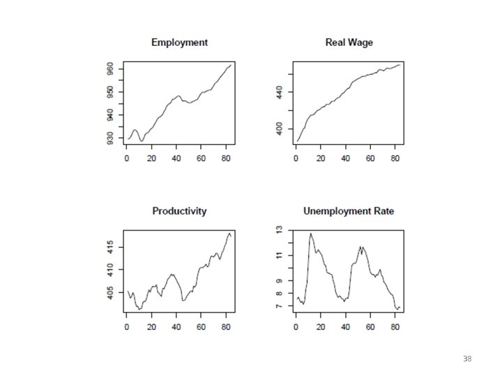
EXAMPLE OF VAR MODELING IN R • “vars” package deals with VAR models. • Let’s consider the Canadian data for an application of the model. • Canadian time series for labour productivity (prod), employment (e), unemployment rate (U) and real wages (rw) (source: OECD database) • Series is quarterly. The sample range is from the 1 st. Q 1980 until ¨ 4 th. Q 2000. 36

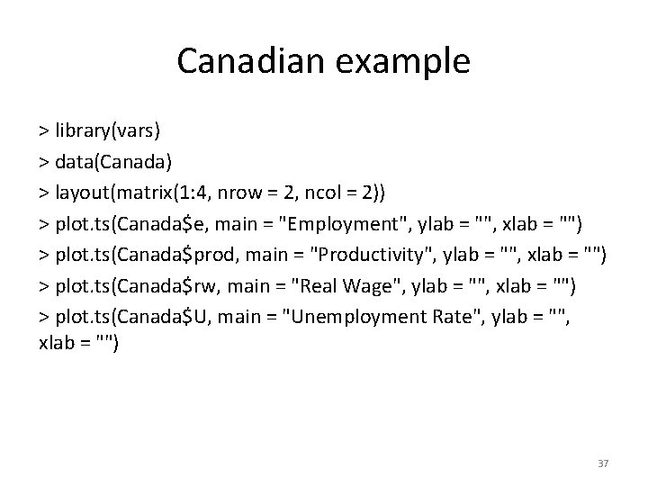
Canadian example > library(vars) > data(Canada) > layout(matrix(1: 4, nrow = 2, ncol = 2)) > plot. ts(Canada$e, main = "Employment", ylab = "", xlab = "") > plot. ts(Canada$prod, main = "Productivity", ylab = "", xlab = "") > plot. ts(Canada$rw, main = "Real Wage", ylab = "", xlab = "") > plot. ts(Canada$U, main = "Unemployment Rate", ylab = "", xlab = "") 37

38

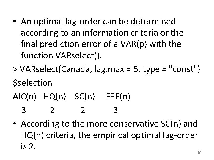
• An optimal lag-order can be determined according to an information criteria or the final prediction error of a VAR(p) with the function VARselect(). > VARselect(Canada, lag. max = 5, type = "const") $selection AIC(n) HQ(n) SC(n) FPE(n) 3 2 2 3 • According to the more conservative SC(n) and HQ(n) criteria, the empirical optimal lag-order is 2. 39

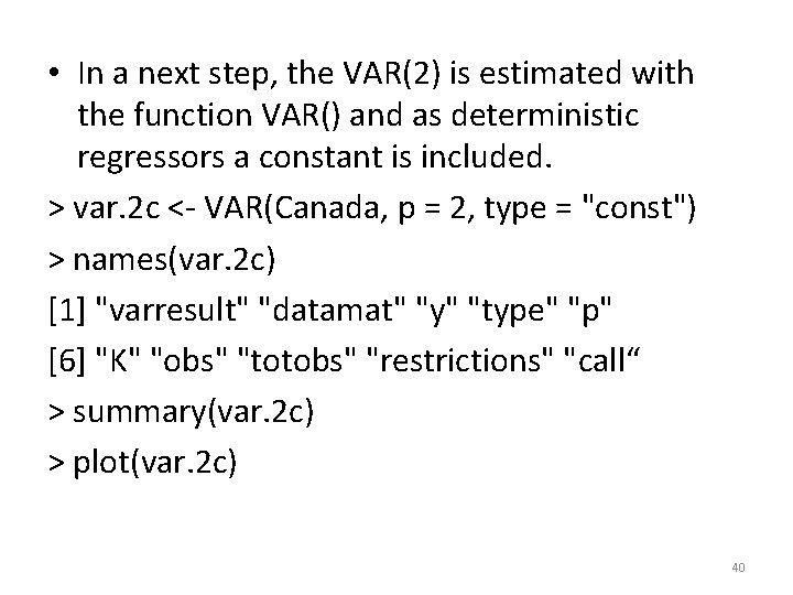
• In a next step, the VAR(2) is estimated with the function VAR() and as deterministic regressors a constant is included. > var. 2 c <- VAR(Canada, p = 2, type = "const") > names(var. 2 c) [1] "varresult" "datamat" "y" "type" "p" [6] "K" "obs" "totobs" "restrictions" "call“ > summary(var. 2 c) > plot(var. 2 c) 40

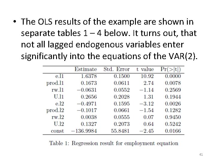
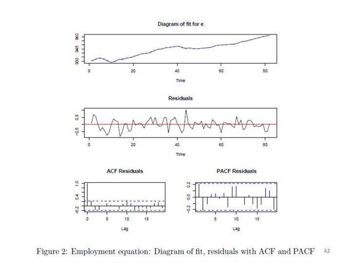
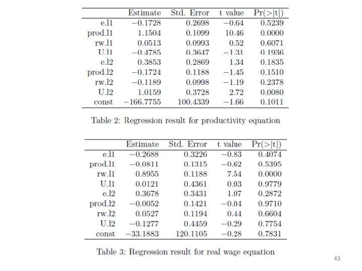
• The OLS results of the example are shown in separate tables 1 – 4 below. It turns out, that not all lagged endogenous variables enter significantly into the equations of the VAR(2). 41

42

43

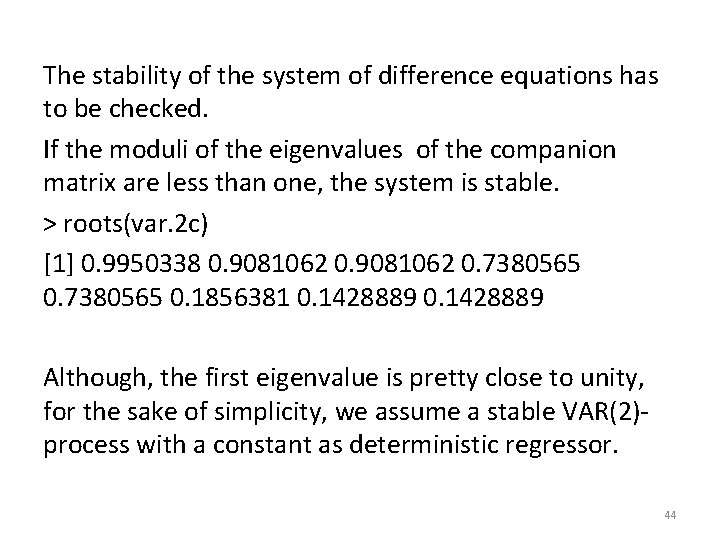
The stability of the system of difference equations has to be checked. If the moduli of the eigenvalues of the companion matrix are less than one, the system is stable. > roots(var. 2 c) [1] 0. 9950338 0. 9081062 0. 7380565 0. 1856381 0. 1428889 Although, the first eigenvalue is pretty close to unity, for the sake of simplicity, we assume a stable VAR(2)process with a constant as deterministic regressor. 44

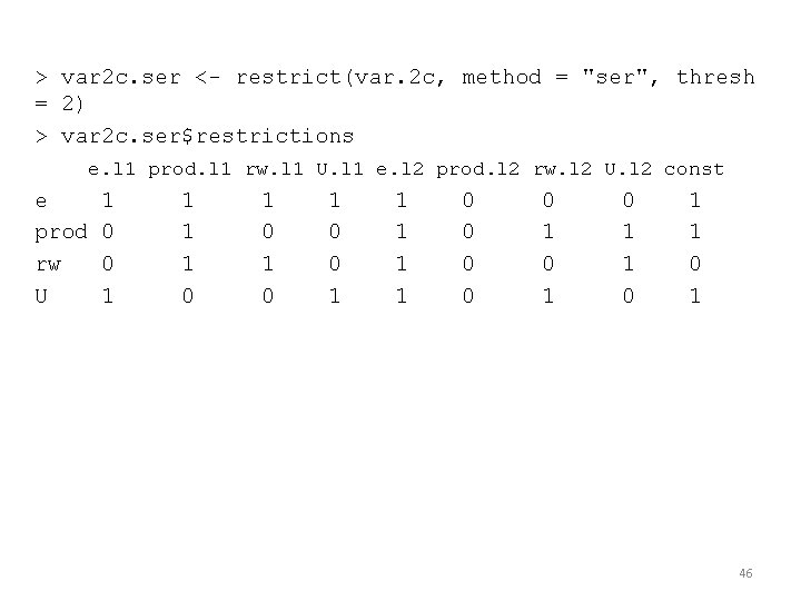
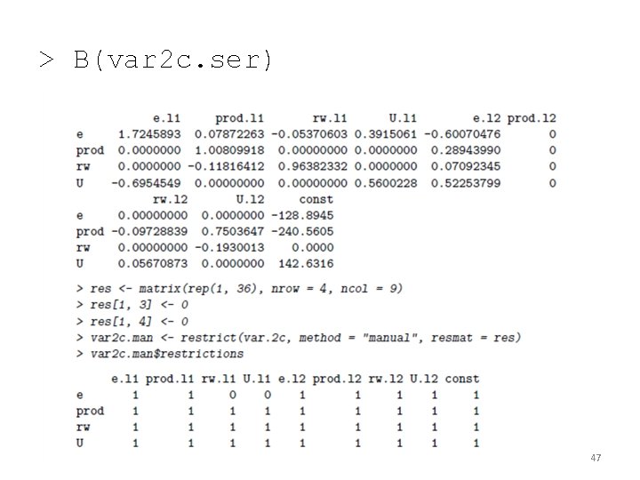
Restricted VARs • From tables 1 -4 it is obvious that not all regressors enter significantly. • With the function restrict() the user has the option to reestimate the VAR either by significance (argument method = ’ser’) or by imposing zero restrictions manually (argument method = ’manual’). • In the former case, each equation is re-estimated separately as long as there are t-values that are in absolute value below the threshold value set by the function’s argument thresh. • In the latter case, a restriction matrix has to be provided that consists of 0/1 values, thereby selecting the coefficients to be retained in the model. The function’s arguments are therefore: 45

> var 2 c. ser <- restrict(var. 2 c, method = "ser", thresh = 2) > var 2 c. ser$restrictions e. l 1 prod. l 1 rw. l 1 U. l 1 e. l 2 prod. l 2 rw. l 2 U. l 2 const e prod rw U 1 0 0 1 1 0 1 0 1 0 0 1 1 1 0 0 0 1 0 1 46

> B(var 2 c. ser) 47

48

49

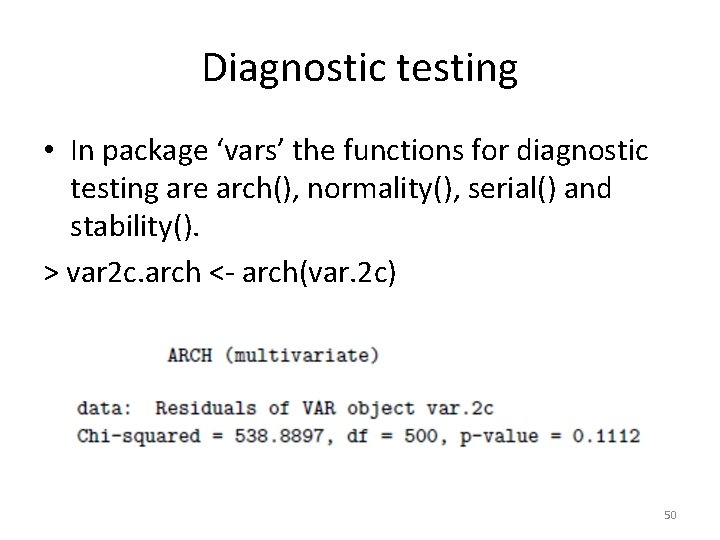
Diagnostic testing • In package ‘vars’ the functions for diagnostic testing are arch(), normality(), serial() and stability(). > var 2 c. arch <- arch(var. 2 c) 50

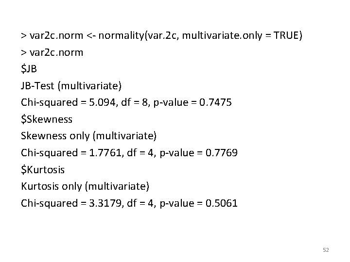
• The Jarque-Bera normality tests for univariate and multivariate series are implemented and applied to the residuals of a VAR(p) as well as separate tests for multivariate skewness and kurtosis (see Bera & Jarque [1980], [1981] and Jarque & Bera [1987] and Lutkepohl [2006]). • The univariate versions of the Jarque-Bera test are applied to the residuals of each equation. • A multivariate version of this test can be computed by using the residuals that are standardized by a Choleski decomposition of the variance-covariance matrix for the centered residuals. 51

> var 2 c. norm <- normality(var. 2 c, multivariate. only = TRUE) > var 2 c. norm $JB JB-Test (multivariate) Chi-squared = 5. 094, df = 8, p-value = 0. 7475 $Skewness only (multivariate) Chi-squared = 1. 7761, df = 4, p-value = 0. 7769 $Kurtosis only (multivariate) Chi-squared = 3. 3179, df = 4, p-value = 0. 5061 52

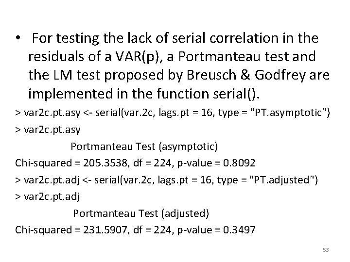
• For testing the lack of serial correlation in the residuals of a VAR(p), a Portmanteau test and the LM test proposed by Breusch & Godfrey are implemented in the function serial(). > var 2 c. pt. asy <- serial(var. 2 c, lags. pt = 16, type = "PT. asymptotic") > var 2 c. pt. asy Portmanteau Test (asymptotic) Chi-squared = 205. 3538, df = 224, p-value = 0. 8092 > var 2 c. pt. adj <- serial(var. 2 c, lags. pt = 16, type = "PT. adjusted") > var 2 c. pt. adj Portmanteau Test (adjusted) Chi-squared = 231. 5907, df = 224, p-value = 0. 3497 53

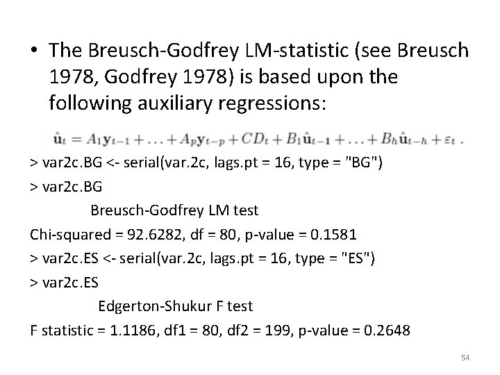
• The Breusch-Godfrey LM-statistic (see Breusch 1978, Godfrey 1978) is based upon the following auxiliary regressions: > var 2 c. BG <- serial(var. 2 c, lags. pt = 16, type = "BG") > var 2 c. BG Breusch-Godfrey LM test Chi-squared = 92. 6282, df = 80, p-value = 0. 1581 > var 2 c. ES <- serial(var. 2 c, lags. pt = 16, type = "ES") > var 2 c. ES Edgerton-Shukur F test F statistic = 1. 1186, df 1 = 80, df 2 = 199, p-value = 0. 2648 54

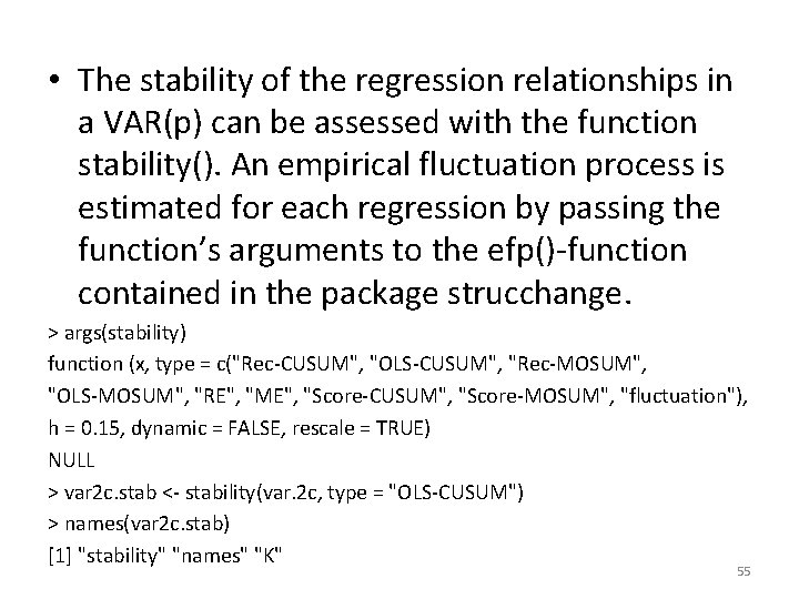
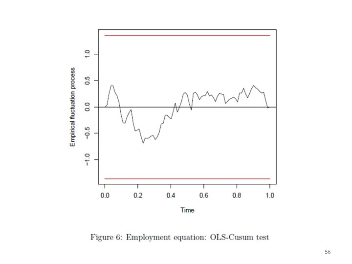
• The stability of the regression relationships in a VAR(p) can be assessed with the function stability(). An empirical fluctuation process is estimated for each regression by passing the function’s arguments to the efp()-function contained in the package strucchange. > args(stability) function (x, type = c("Rec-CUSUM", "OLS-CUSUM", "Rec-MOSUM", "OLS-MOSUM", "RE", "ME", "Score-CUSUM", "Score-MOSUM", "fluctuation"), h = 0. 15, dynamic = FALSE, rescale = TRUE) NULL > var 2 c. stab <- stability(var. 2 c, type = "OLS-CUSUM") > names(var 2 c. stab) [1] "stability" "names" "K" 55

56

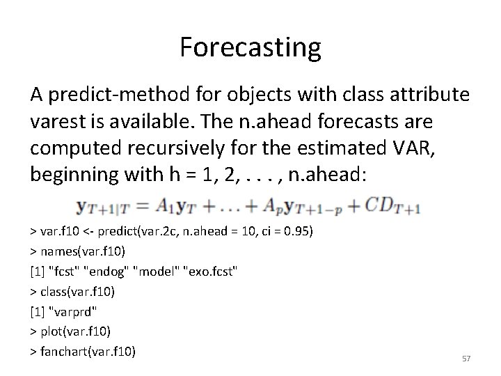
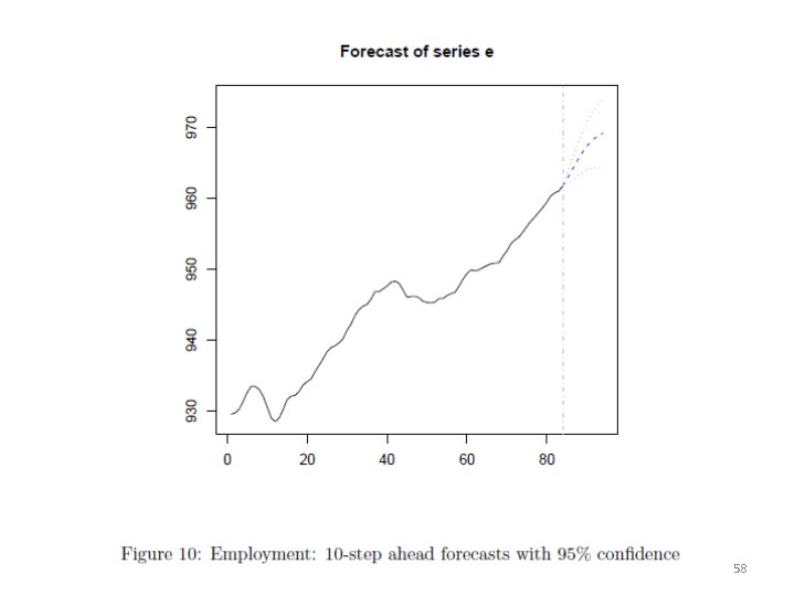
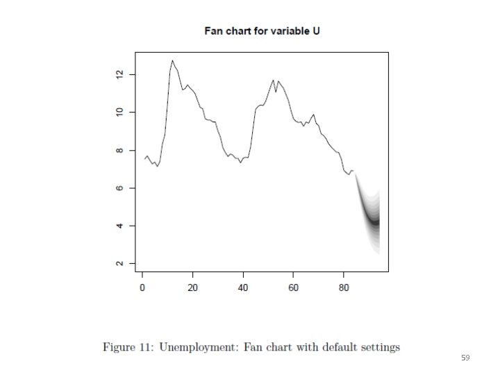
Forecasting A predict-method for objects with class attribute varest is available. The n. ahead forecasts are computed recursively for the estimated VAR, beginning with h = 1, 2, . . . , n. ahead: > var. f 10 <- predict(var. 2 c, n. ahead = 10, ci = 0. 95) > names(var. f 10) [1] "fcst" "endog" "model" "exo. fcst" > class(var. f 10) [1] "varprd" > plot(var. f 10) > fanchart(var. f 10) 57

58

59

GRANGER CAUSALITY • In time series analysis, sometimes, we would like to know whether changes in a variable will have an impact on changes other variables. • To find out this phenomena more accurately, we need to learn more about Granger Causality Test. 60

GRANGER CAUSALITY • In principle, the concept is as follows: • If X causes Y, then, changes of X happened first then followed by changes of Y. 61

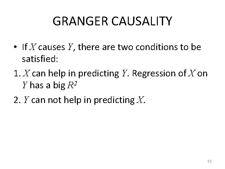
GRANGER CAUSALITY • If X causes Y, there are two conditions to be satisfied: 1. X can help in predicting Y. Regression of X on Y has a big R 2 2. Y can not help in predicting X. 62

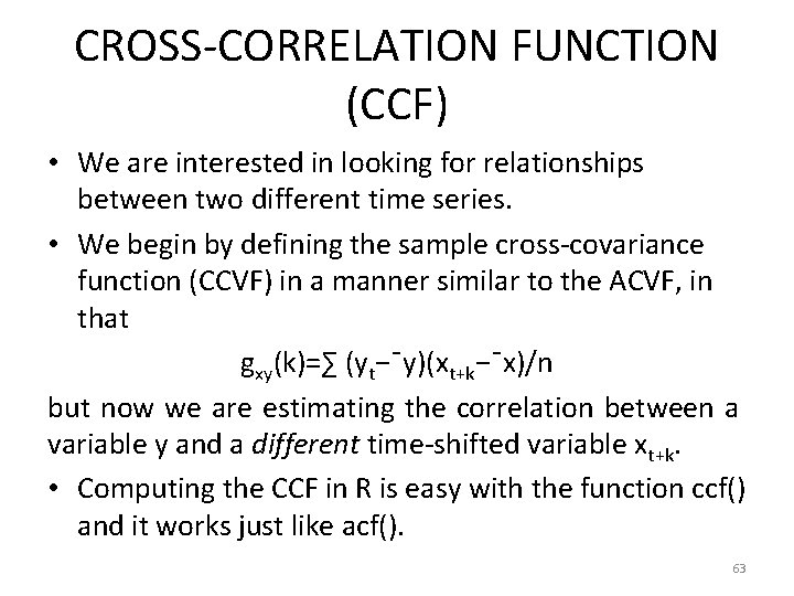
CROSS-CORRELATION FUNCTION (CCF) • We are interested in looking for relationships between two different time series. • We begin by defining the sample cross-covariance function (CCVF) in a manner similar to the ACVF, in that gxy(k)=∑ (yt−¯y)(xt+k−¯x)/n but now we are estimating the correlation between a variable y and a different time-shifted variable xt+k. • Computing the CCF in R is easy with the function ccf() and it works just like acf(). 63

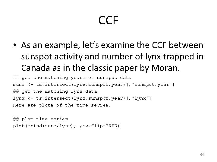
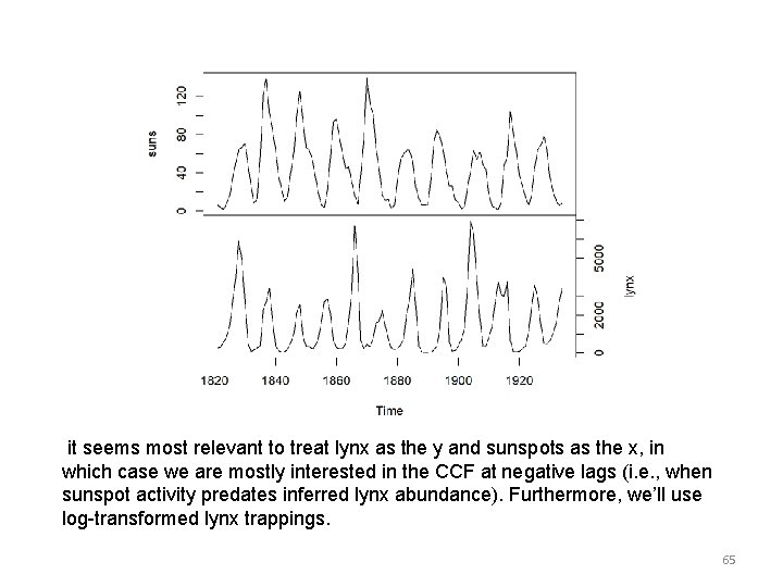
CCF • As an example, let’s examine the CCF between sunspot activity and number of lynx trapped in Canada as in the classic paper by Moran. ## get the matching years of sunspot data suns <- ts. intersect(lynx, sunspot. year)[, "sunspot. year"] ## get the matching lynx data lynx <- ts. intersect(lynx, sunspot. year)[, "lynx"] Here are plots of the time series. ## plot time series plot(cbind(suns, lynx), yax. flip=TRUE) 64

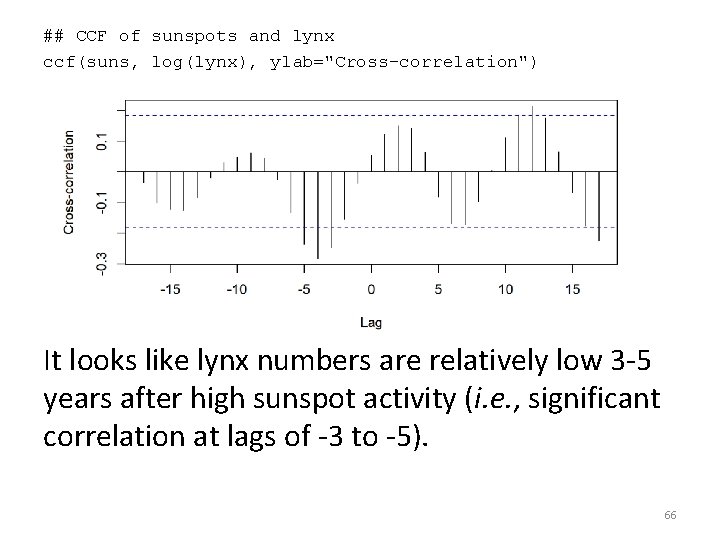
it seems most relevant to treat lynx as the y and sunspots as the x, in which case we are mostly interested in the CCF at negative lags (i. e. , when sunspot activity predates inferred lynx abundance). Furthermore, we’ll use log-transformed lynx trappings. 65

## CCF of sunspots and lynx ccf(suns, log(lynx), ylab="Cross-correlation") It looks like lynx numbers are relatively low 3 -5 years after high sunspot activity (i. e. , significant correlation at lags of -3 to -5). 66

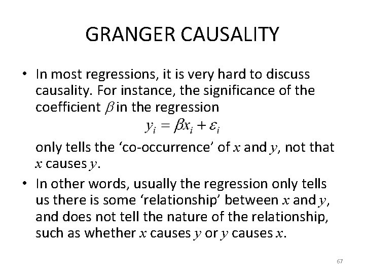
GRANGER CAUSALITY • In most regressions, it is very hard to discuss causality. For instance, the significance of the coefficient in the regression only tells the ‘co-occurrence’ of x and y, not that x causes y. • In other words, usually the regression only tells us there is some ‘relationship’ between x and y, and does not tell the nature of the relationship, such as whether x causes y or y causes x. 67

GRANGER CAUSALITY • One good thing of time series vector autoregression is that we could test ‘causality’ in some sense. This test is first proposed by Granger (1969), and therefore we refer it Granger causality. • We will restrict our discussion to a system of two variables, x and y. y is said to Granger-cause x if current or lagged values of y helps to predict future values of x. On the other hand, y fails to Granger-cause x if for all s > 0, the mean squared error of a forecast of xt+s based on (xt, xt− 1, . . . ) is the same as that is based on (yt, yt− 1, . . . ) and (xt, xt− 1, . . . ). 68

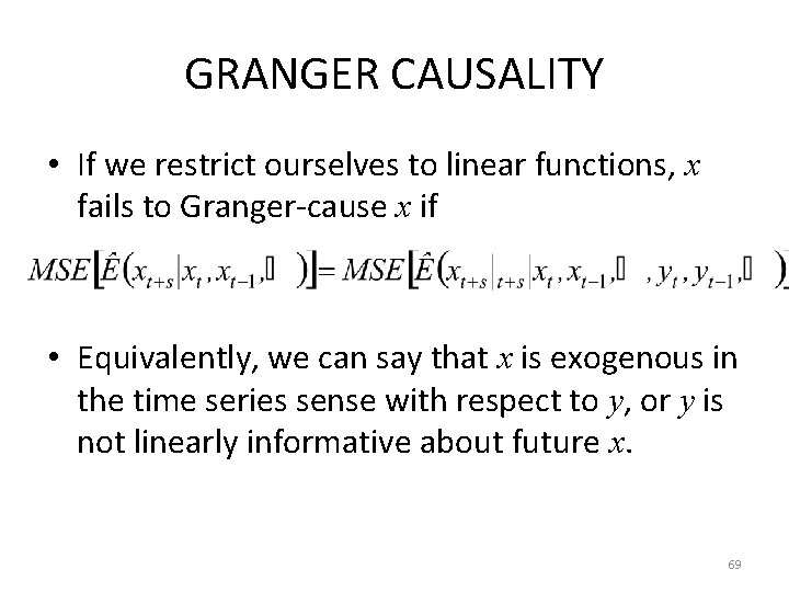
GRANGER CAUSALITY • If we restrict ourselves to linear functions, x fails to Granger-cause x if • Equivalently, we can say that x is exogenous in the time series sense with respect to y, or y is not linearly informative about future x. 69

GRANGER CAUSALITY • A variable X is said to Granger cause another variable Y, if Y can be better predicted from the past of X and Y together than the past of Y alone, other relevant information being used in the prediction (Pierce, 1977). 70

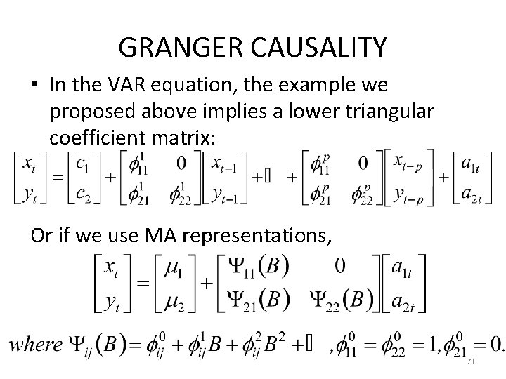
GRANGER CAUSALITY • In the VAR equation, the example we proposed above implies a lower triangular coefficient matrix: Or if we use MA representations, 71

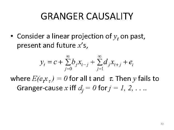
GRANGER CAUSALITY • Consider a linear projection of yt on past, present and future x’s, where E(etx ) = 0 for all t and . Then y fails to Granger-cause x iff dj = 0 for j = 1, 2, . . 72

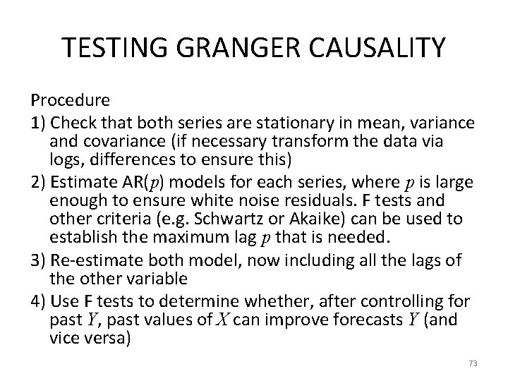
TESTING GRANGER CAUSALITY Procedure 1) Check that both series are stationary in mean, variance and covariance (if necessary transform the data via logs, differences to ensure this) 2) Estimate AR(p) models for each series, where p is large enough to ensure white noise residuals. F tests and other criteria (e. g. Schwartz or Akaike) can be used to establish the maximum lag p that is needed. 3) Re-estimate both model, now including all the lags of the other variable 4) Use F tests to determine whether, after controlling for past Y, past values of X can improve forecasts Y (and vice versa) 73

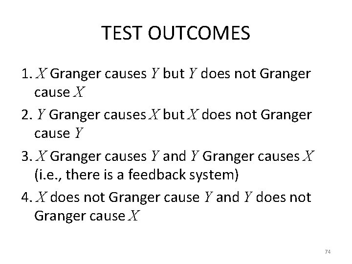
TEST OUTCOMES 1. X Granger causes Y but Y does not Granger cause X 2. Y Granger causes X but X does not Granger cause Y 3. X Granger causes Y and Y Granger causes X (i. e. , there is a feedback system) 4. X does not Granger cause Y and Y does not Granger cause X 74

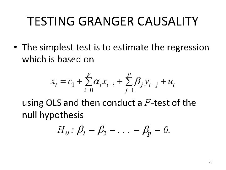
TESTING GRANGER CAUSALITY • The simplest test is to estimate the regression which is based on using OLS and then conduct a F-test of the null hypothesis H 0 : 1 = 2 =. . . = p = 0. 75

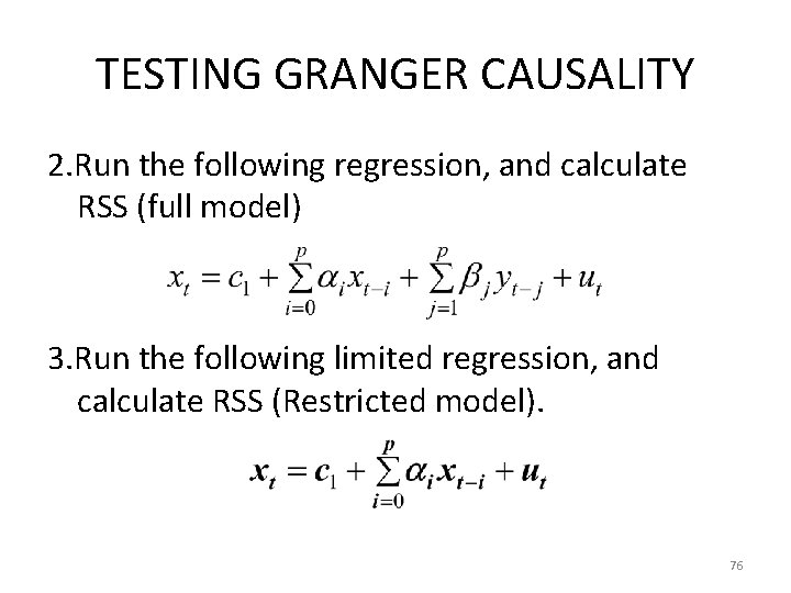
TESTING GRANGER CAUSALITY 2. Run the following regression, and calculate RSS (full model) 3. Run the following limited regression, and calculate RSS (Restricted model). 76

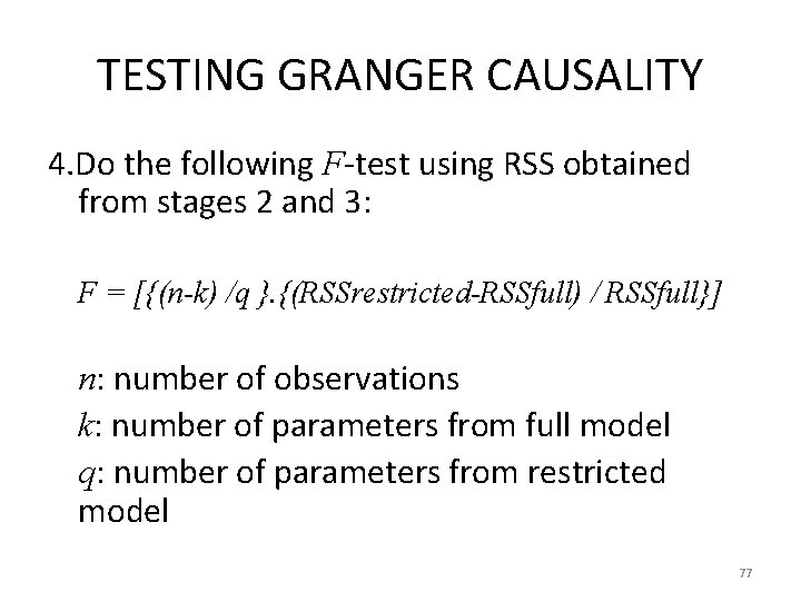
TESTING GRANGER CAUSALITY 4. Do the following F-test using RSS obtained from stages 2 and 3: F = [{(n-k) /q }. {(RSSrestricted-RSSfull) / RSSfull}] n: number of observations k: number of parameters from full model q: number of parameters from restricted model 77

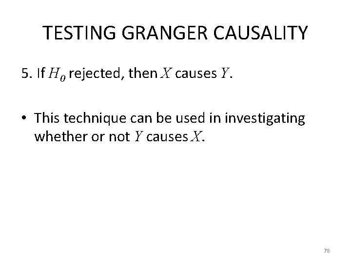
TESTING GRANGER CAUSALITY 5. If H 0 rejected, then X causes Y. • This technique can be used in investigating whether or not Y causes X. 78

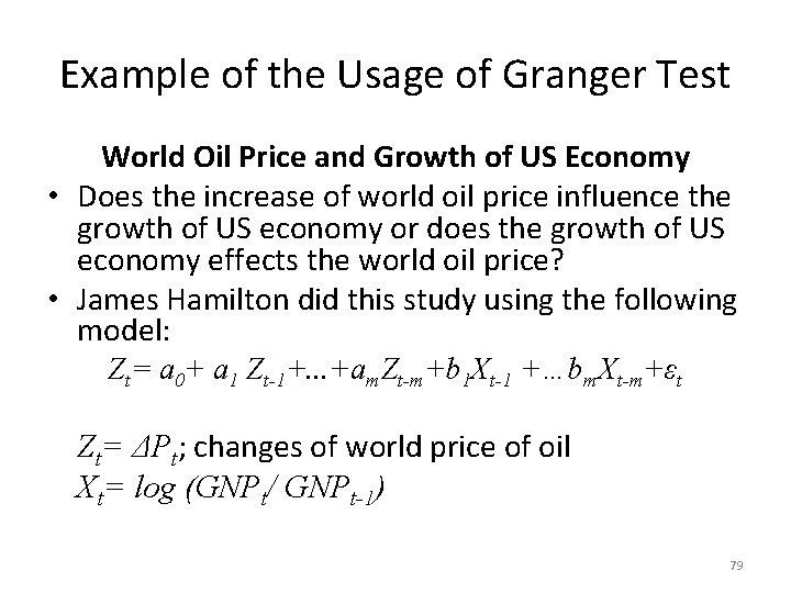
Example of the Usage of Granger Test World Oil Price and Growth of US Economy • Does the increase of world oil price influence the growth of US economy or does the growth of US economy effects the world oil price? • James Hamilton did this study using the following model: Zt= a 0+ a 1 Zt-1+. . . +am. Zt-m+b 1 Xt-1 +…bm. Xt-m+εt Zt= ΔPt; changes of world price of oil Xt= log (GNPt/ GNPt-1) 79

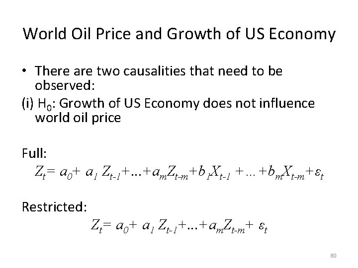
World Oil Price and Growth of US Economy • There are two causalities that need to be observed: (i) H 0: Growth of US Economy does not influence world oil price Full: Zt= a 0+ a 1 Zt-1+. . . +am. Zt-m+b 1 Xt-1 +…+bm. Xt-m+εt Restricted: Zt= a 0+ a 1 Zt-1+. . . +am. Zt-m+ εt 80

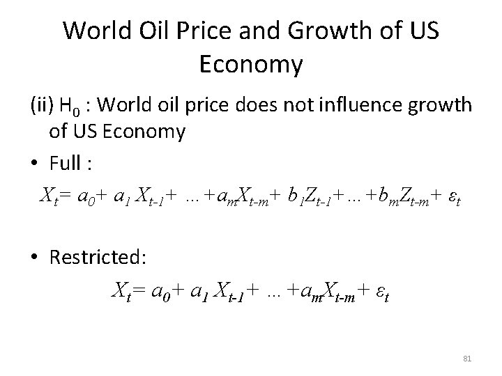
World Oil Price and Growth of US Economy (ii) H 0 : World oil price does not influence growth of US Economy • Full : Xt= a 0+ a 1 Xt-1+ …+am. Xt-m+ b 1 Zt-1+…+bm. Zt-m+ εt • Restricted: Xt= a 0+ a 1 Xt-1+ …+am. Xt-m+ εt 81

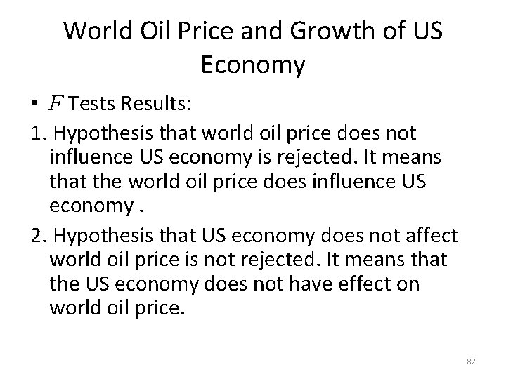
World Oil Price and Growth of US Economy • F Tests Results: 1. Hypothesis that world oil price does not influence US economy is rejected. It means that the world oil price does influence US economy. 2. Hypothesis that US economy does not affect world oil price is not rejected. It means that the US economy does not have effect on world oil price. 82

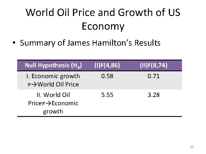
World Oil Price and Growth of US Economy • Summary of James Hamilton’s Results Null Hypothesis (H 0) (I)F(4, 86) (II)F(8, 74) I. Economic growth ≠→World Oil Price 0. 58 0. 71 II. World Oil Price≠→Economic growth 5. 55 3. 28 83

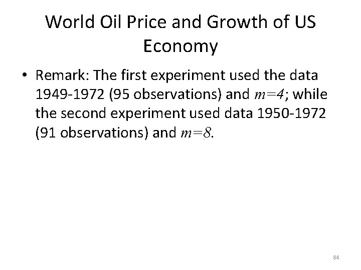
World Oil Price and Growth of US Economy • Remark: The first experiment used the data 1949 -1972 (95 observations) and m=4; while the second experiment used data 1950 -1972 (91 observations) and m=8. 84

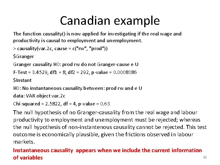
Canadian example The function causality() is now applied for investigating if the real wage and productivity is causal to employment and unemployment. > causality(var. 2 c, cause = c("rw", "prod")) $Granger causality H 0: prod rw do not Granger-cause e U F-Test = 3. 4529, df 1 = 8, df 2 = 292, p-value = 0. 0008086 $Instant H 0: No instantaneous causality between: prod rw and e U data: VAR object var. 2 c Chi-squared = 2. 5822, df = 4, p-value = 0. 63 The null hypothesis of no Granger-causality from the real wage and labour productivity to employment and unemployment must be rejected; whereas the null hypothesis of non-instantenous causality cannot be rejected. This test outcome is economically plausible, given the frictions observed in labour markets. Instantaneous causality appears when we include the current information 85 of variables

Chicken vs. Egg • This causality test is also can be used in explaining which comes first: chicken or egg. More specifically, the test can be used in testing whether the existence of egg causes the existence of chicken or vise versa. • Thurman and Fisher did this study using yearly data of chicken population and egg productions in the US from 1930 to 1983 • The results: 1. Egg causes the chicken. 2. There is no evidence that chicken causes egg. 86

Chicken vs. Egg • Remark: Hypothesis that egg has no effect on chicken population is rejected; while the other hypothesis that chicken has no effect on egg is not rejected. Why? 87

GRANGER CAUSALITY • We have to be aware of that Granger causality does not equal to what we usually mean by causality. For instance, even if x 1 does not cause x 2, it may still help to predict x 2, and thus Granger-causes x 2 if changes in x 1 precedes that of x 2 for some reason. • A naive example is that we observe that a dragonfly flies much lower before a rain storm, due to the lower air pressure. We know that dragonflies do not cause a rain storm, but it does help to predict a rain storm, thus Granger-causes a rain storm. 88