STAT 497 LECTURE NOTES 5 UNIT ROOT TESTS

STAT 497 LECTURE NOTES 5 UNIT ROOT TESTS 1

UNIT ROOTS IN TIME SERIES MODELS • Shock is usually used to describe an unexpected change in a variable or in the value of the error terms at a particular time period. • When we have a stationary system, effect of a shock will die out gradually. • When we have a non-stationary system, effect of a shock is permanent. 2

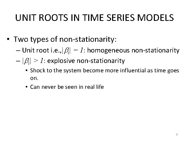
UNIT ROOTS IN TIME SERIES MODELS • Two types of non-stationarity: – Unit root i. e. , | i| = 1: homogeneous non-stationarity – | i| > 1: explosive non-stationarity • Shock to the system become more influential as time goes on. • Can never be seen in real life 3

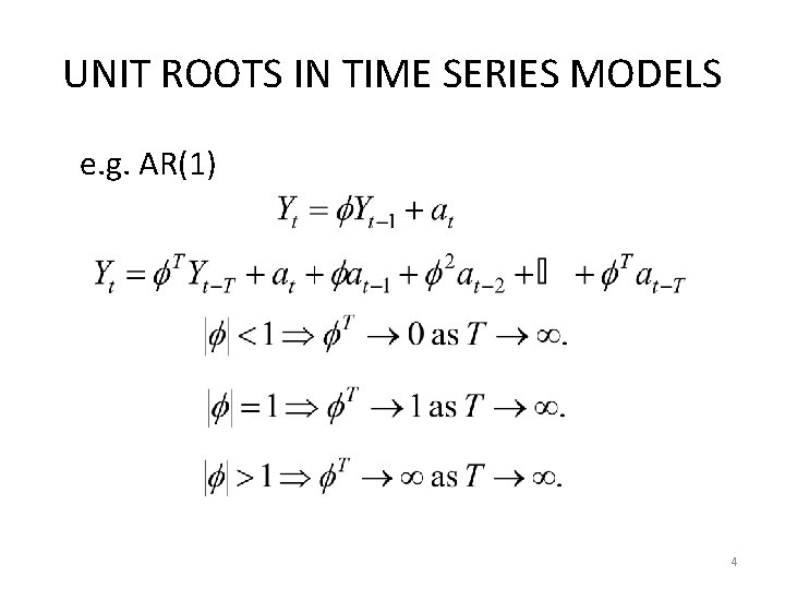
UNIT ROOTS IN TIME SERIES MODELS e. g. AR(1) 4

UNIT ROOTS IN TIME SERIES MODELS • A root near 1 of the AR polynomial differencing • A root near 1 of the MA polynomial over-differencing 5

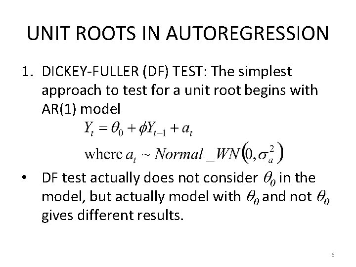
UNIT ROOTS IN AUTOREGRESSION 1. DICKEY-FULLER (DF) TEST: The simplest approach to test for a unit root begins with AR(1) model • DF test actually does not consider 0 in the model, but actually model with 0 and not 0 gives different results. 6

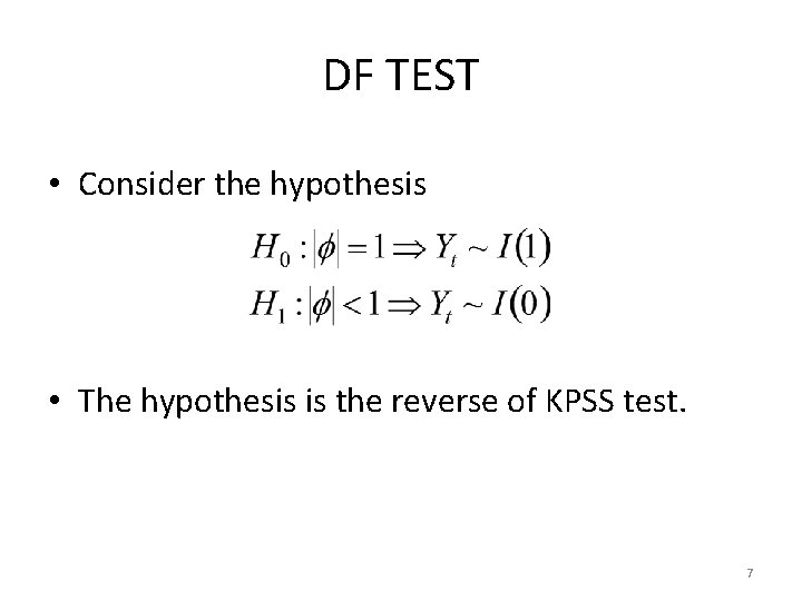
DF TEST • Consider the hypothesis • The hypothesis is the reverse of KPSS test. 7

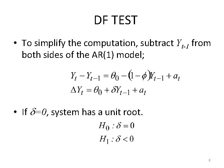
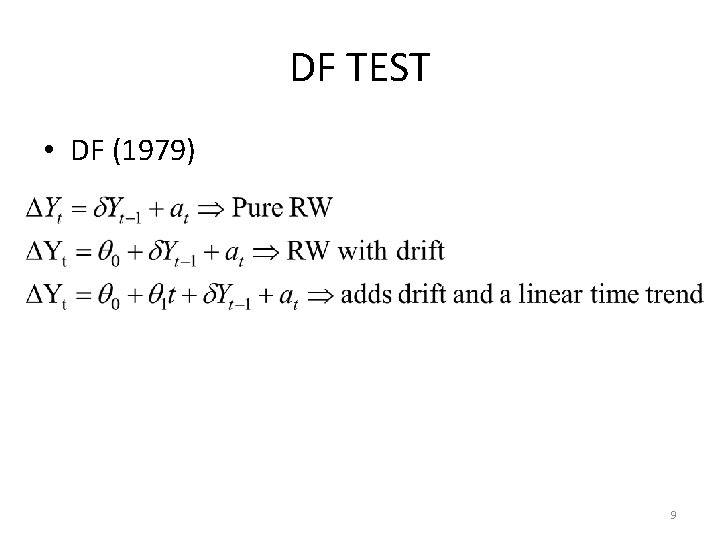
DF TEST • To simplify the computation, subtract Yt-1 from both sides of the AR(1) model; • If =0, system has a unit root. 8

DF TEST • DF (1979) 9

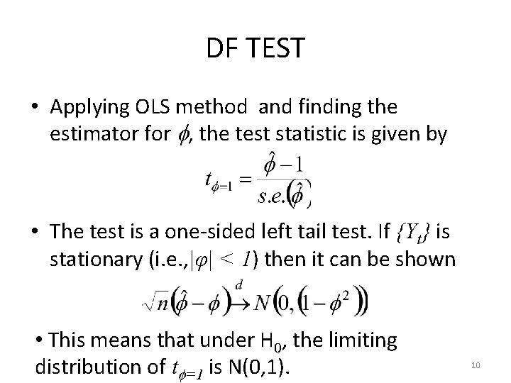
DF TEST • Applying OLS method and finding the estimator for , the test statistic is given by • The test is a one-sided left tail test. If {Yt} is stationary (i. e. , |φ| < 1) then it can be shown • This means that under H 0, the limiting distribution of t =1 is N(0, 1). 10

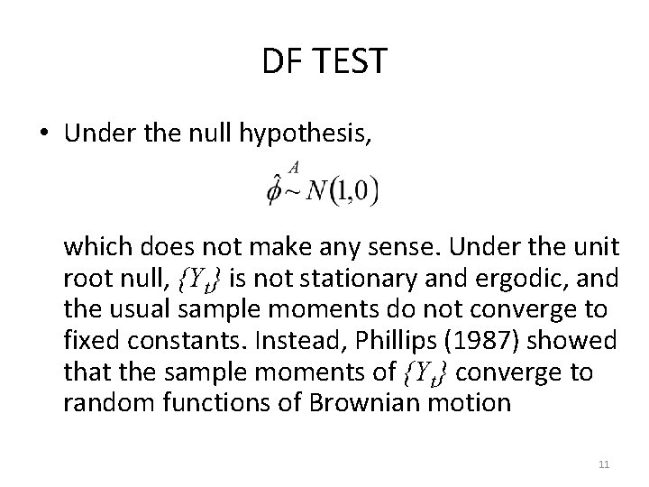
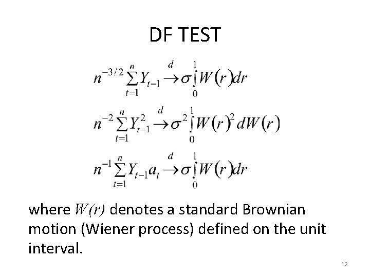
DF TEST • Under the null hypothesis, which does not make any sense. Under the unit root null, {Yt} is not stationary and ergodic, and the usual sample moments do not converge to fixed constants. Instead, Phillips (1987) showed that the sample moments of {Yt} converge to random functions of Brownian motion 11

DF TEST where W(r) denotes a standard Brownian motion (Wiener process) defined on the unit interval. 12

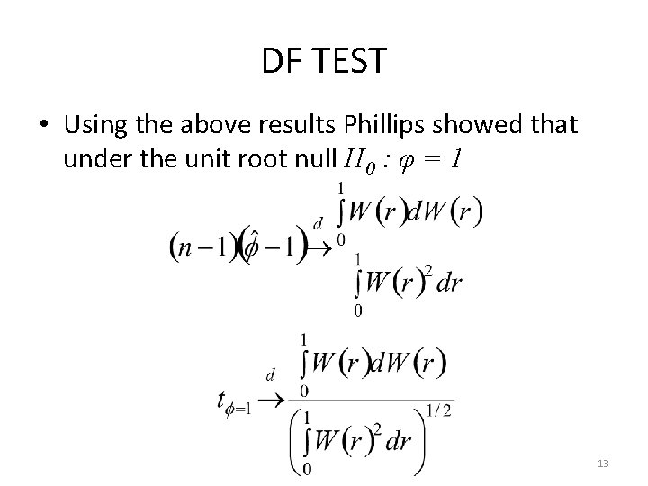
DF TEST • Using the above results Phillips showed that under the unit root null H 0 : φ = 1 13

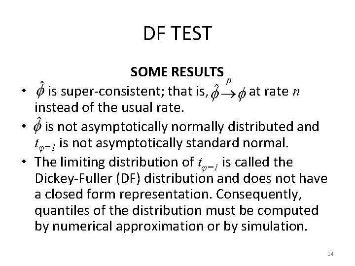
DF TEST SOME RESULTS • is super-consistent; that is, at rate n instead of the usual rate. • is not asymptotically normally distributed and tφ=1 is not asymptotically standard normal. • The limiting distribution of tφ=1 is called the Dickey-Fuller (DF) distribution and does not have a closed form representation. Consequently, quantiles of the distribution must be computed by numerical approximation or by simulation. 14

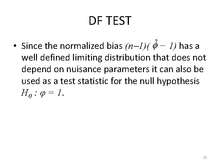
DF TEST • Since the normalized bias (n 1)( − 1) has a well defined limiting distribution that does not depend on nuisance parameters it can also be used as a test statistic for the null hypothesis H 0 : φ = 1. 15

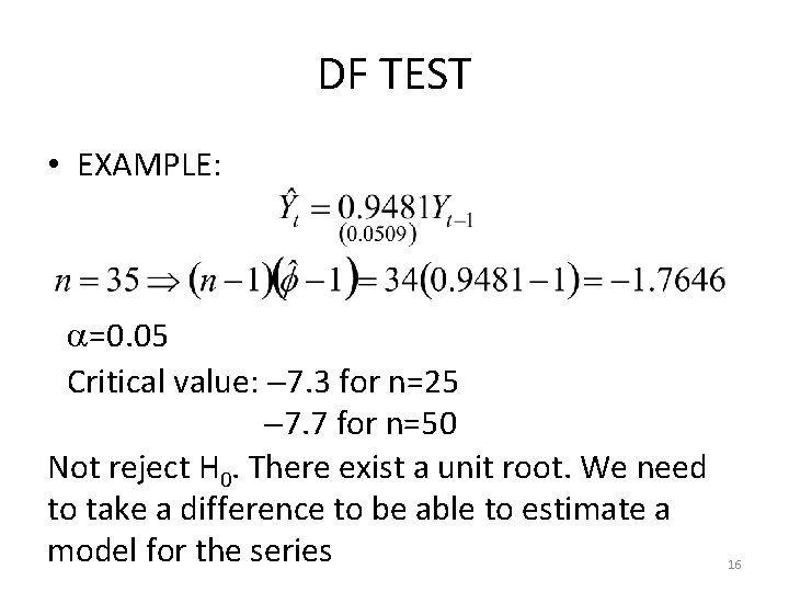
DF TEST • EXAMPLE: =0. 05 Critical value: 7. 3 for n=25 7. 7 for n=50 Not reject H 0. There exist a unit root. We need to take a difference to be able to estimate a model for the series 16

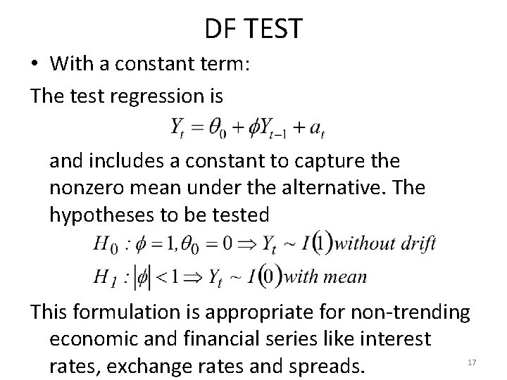
DF TEST • With a constant term: The test regression is and includes a constant to capture the nonzero mean under the alternative. The hypotheses to be tested This formulation is appropriate for non-trending economic and financial series like interest rates, exchange rates and spreads. 17

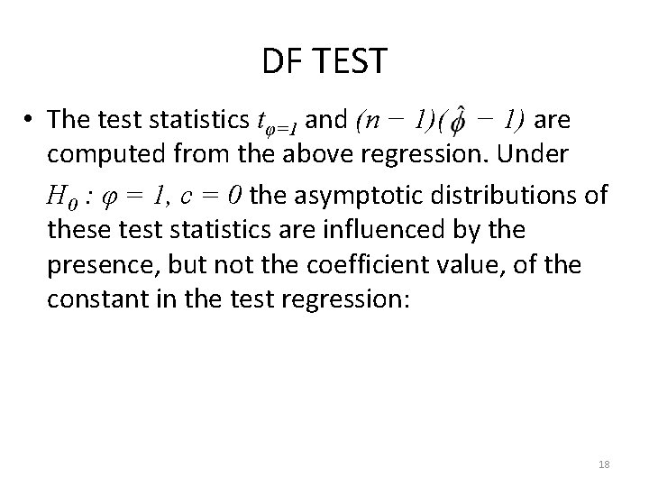
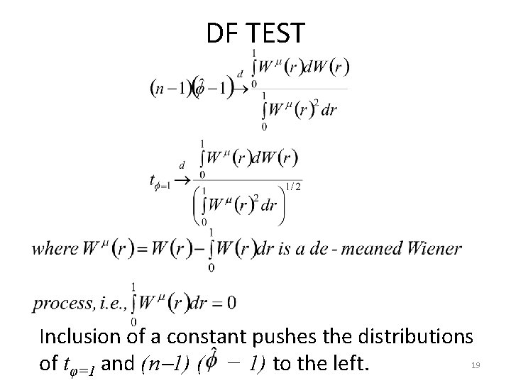
DF TEST • The test statistics tφ=1 and (n − 1)( − 1) are computed from the above regression. Under H 0 : φ = 1, c = 0 the asymptotic distributions of these test statistics are influenced by the presence, but not the coefficient value, of the constant in the test regression: 18

DF TEST Inclusion of a constant pushes the distributions of tφ=1 and (n 1) ( − 1) to the left. 19

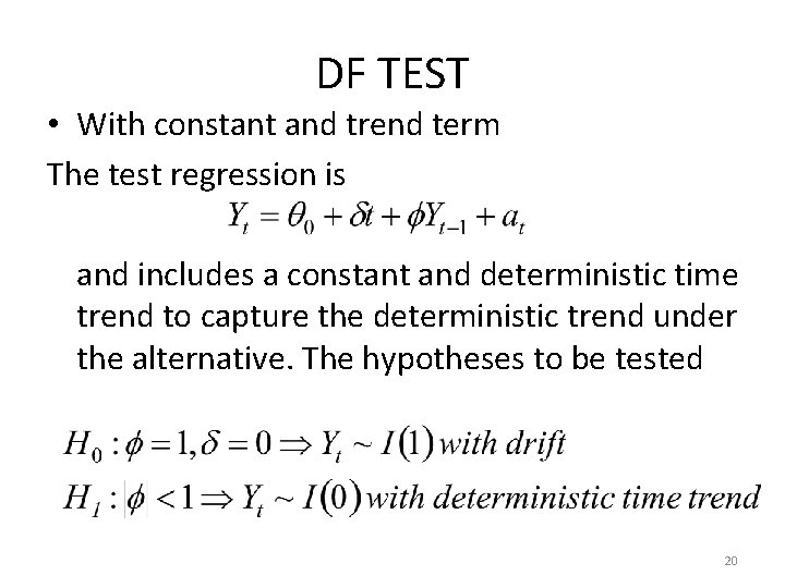
DF TEST • With constant and trend term The test regression is and includes a constant and deterministic time trend to capture the deterministic trend under the alternative. The hypotheses to be tested 20

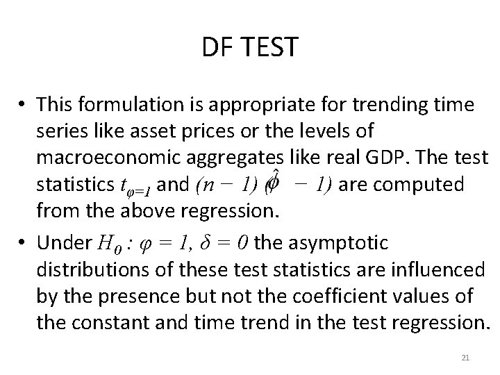
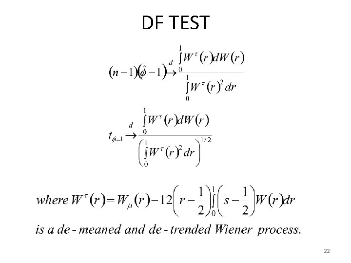
DF TEST • This formulation is appropriate for trending time series like asset prices or the levels of macroeconomic aggregates like real GDP. The test statistics tφ=1 and (n − 1) ( − 1) are computed from the above regression. • Under H 0 : φ = 1, δ = 0 the asymptotic distributions of these test statistics are influenced by the presence but not the coefficient values of the constant and time trend in the test regression. 21

DF TEST 22

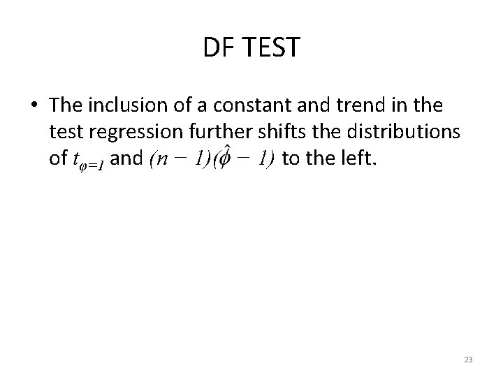
DF TEST • The inclusion of a constant and trend in the test regression further shifts the distributions of tφ=1 and (n − 1)( − 1) to the left. 23

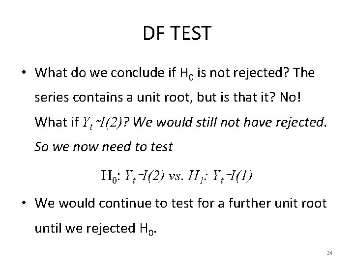
DF TEST • What do we conclude if H 0 is not rejected? The series contains a unit root, but is that it? No! What if Yt∼I(2)? We would still not have rejected. So we now need to test H 0: Yt∼I(2) vs. H 1: Yt∼I(1) • We would continue to test for a further unit root until we rejected H 0. 24

DF TEST • This test is valid only if at is WN. If there is a serial correlation, the test should be augmented. So, check for possible autoregression in at. • Many economic and financial time series have a more complicated dynamic structure than is captured by a simple AR(1) model. • Said and Dickey (1984) augment the basic autoregressive unit root test to accommodate general ARMA(p, q) models with unknown orders and their test is referred to as the augmented Dickey - Fuller (ADF) test. 25

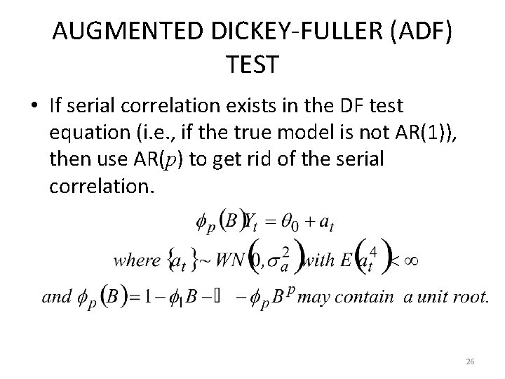
AUGMENTED DICKEY-FULLER (ADF) TEST • If serial correlation exists in the DF test equation (i. e. , if the true model is not AR(1)), then use AR(p) to get rid of the serial correlation. 26

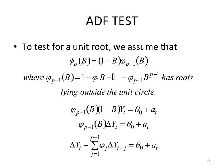
ADF TEST • To test for a unit root, we assume that 27

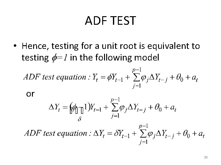
ADF TEST • Hence, testing for a unit root is equivalent to testing =1 in the following model or 28

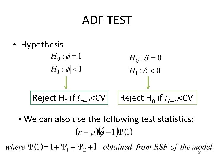
ADF TEST • Hypothesis Reject H 0 if t =1<CV Reject H 0 if t =0<CV • We can also use the following test statistics: 29

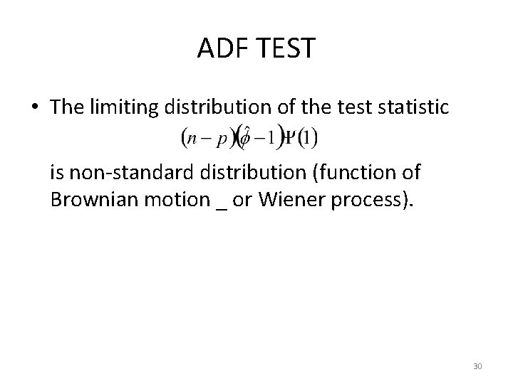
ADF TEST • The limiting distribution of the test statistic is non-standard distribution (function of Brownian motion _ or Wiener process). 30

Choosing the Lag Length for the ADF Test • An important practical issue for the implementation of the ADF test is the specification of the lag length p. If p is too small, then the remaining serial correlation in the errors will bias the test. If p is too large, then the power of the test will suffer. 31

Choosing the Lag Length for the ADF Test • Ng and Perron (1995) suggest the following data dependent lag length selection procedure that results in stable size of the test and minimal power loss: • First, set an upper bound pmax for p. Next, estimate the ADF test regression with p = pmax. If the absolute value of the t-statistic for testing the significance of the last lagged difference is greater than 1. 6, then set p = pmax and perform the unit root test. Otherwise, reduce the lag length by one and repeat the process. 32

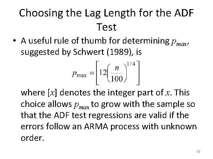
Choosing the Lag Length for the ADF Test • A useful rule of thumb for determining pmax, suggested by Schwert (1989), is where [x] denotes the integer part of x. This choice allows pmax to grow with the sample so that the ADF test regressions are valid if the errors follow an ARMA process with unknown order. 33

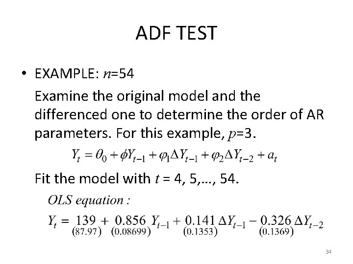
ADF TEST • EXAMPLE: n=54 Examine the original model and the differenced one to determine the order of AR parameters. For this example, p=3. Fit the model with t = 4, 5, …, 54. 34

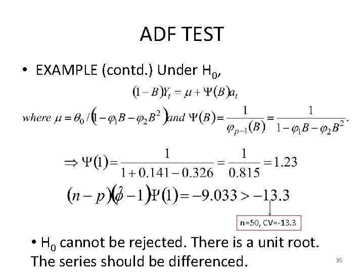
ADF TEST • EXAMPLE (contd. ) Under H 0, n=50, CV=-13. 3 • H 0 cannot be rejected. There is a unit root. The series should be differenced. 35

ADF TEST • If the test statistics is positive, you can automatically decide to not reject the null hypothesis of unit root. • Augmented model can be extended to allow MA terms in at. It is generally believed that MA terms are present in many macroeconomic time series after differencing. Said and Dickey (1984) developed an approach in which the orders of the AR and MA components in the error terms are unknown, but can be approximated by an AR(k) process where k is large enough to allow good approximation to the unknown ARMA(p, q) process. 36

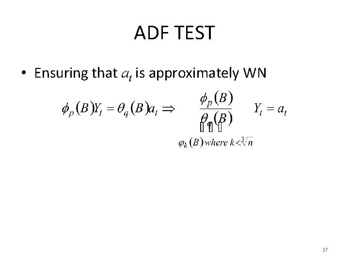
ADF TEST • Ensuring that at is approximately WN 37

PHILLIPS-PERRON (PP) UNIT ROOT TEST • Phillips and Perron (1988) have developed a more comprehensive theory of unit root nonstationarity. The tests are similar to ADF tests. The Phillips-Perron (PP) unit root tests differ from the ADF tests mainly in how they deal with serial correlation and heteroskedasticity in the errors. In particular, where the ADF tests use a parametric autoregression to approximate the ARMA structure of the errors in the test regression, the PP tests ignore any serial correlation in the test regression. • The tests usually give the same conclusions as the ADF tests, and the calculation of the test statistics is complex. 38

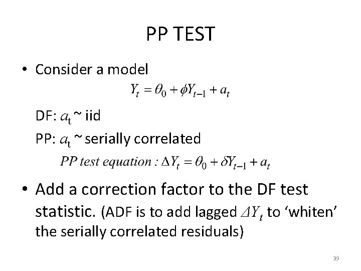
PP TEST • Consider a model DF: at ~ iid PP: at ~ serially correlated • Add a correction factor to the DF test statistic. (ADF is to add lagged ΔYt to ‘whiten’ the serially correlated residuals) 39

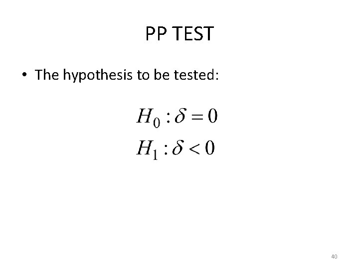
PP TEST • The hypothesis to be tested: 40

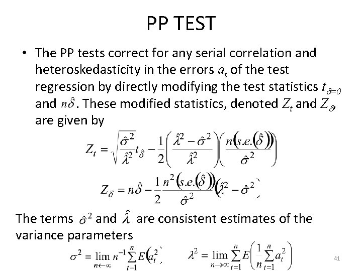
PP TEST • The PP tests correct for any serial correlation and heteroskedasticity in the errors at of the test regression by directly modifying the test statistics t =0 and. These modified statistics, denoted Zt and Z , are given by The terms and are consistent estimates of the variance parameters 41

PP TEST • Under the null hypothesis that = 0, the PP Zt and Z statistics have the same asymptotic distributions as the ADF t-statistic and normalized bias statistics. • One advantage of the PP tests over the ADF tests is that the PP tests are robust to general forms of heteroskedasticity in the error term at. Another advantage is that the user does not have to specify a lag length for the test regression. 42

PROBLEM OF PP TEST • On the other hand, the PP tests tend to be more powerful but, also subject to more severe size distortions – Size problem: actual size is larger than the nominal one when autocorrelations of at are negative. – more sensitive to model misspecification (the order of autoregressive and moving average components). • Plotting ACFs help us to detect the potential size problem – Economic time series sometimes have negative autocorrelations especially at lag one, we can use a Monte Carlo analysis to simulate the appropriate critical values, which may not be attractive to do. 43

Criticism of Dickey-Fuller and Phillips-Perron Type Tests • Main criticism is that the power of the tests is low if the process is stationary but with a root close to the non-stationary boundary. • e. g. the tests are poor at deciding if φ=1 or φ=0. 95, especially with small sample sizes. • If the true data generating process (dgp) is Yt= 0. 95 Yt-1+ at then the null hypothesis of a unit root should be rejected. • One way to get around this is to use a stationarity test (like KPSS test) as well as the unit root tests we have looked at (like ADF or PP). 44

Criticism of Dickey-Fuller and Phillips-Perron Type Tests • The ADF and PP unit root tests are known (from MC simulations) to suffer potentially severe finite sample power and size problems. 1. Power – The ADF and PP tests are known to have low power against the alternative hypothesis that the series is stationary (or TS) with a large autoregressive root. (See, e. g. , De. Jong, et al, J. of Econometrics, 1992. ) 2. Size – The ADF and PP tests are known to have severe size distortion (in the direction of over-rejecting the null) when the series has a large negative moving average root. (See, e. g. , Schwert. JBES, 1989: MA = -0. 8, size = 100%!) 45

Criticism of Dickey-Fuller and Phillips-Perron Type Tests • A variety of alternative procedures have been proposed that try to resolve these problems, particularly, the power problem, but the ADF and PP tests continue to be the most widely used unit root tests. That may be changing! 46

STRUCTURAL BREAKS • A stationary time-series may look like nonstationary when there are structural breaks in the intercept or trend • The unit root tests lead to false non-rejection of the null when we don’t consider the structural breaks low power • A single breakpoint is introduced in Perron (1989) into the regression model; Perron (1997) extended it to a case of unknown breakpoint • Perron, P. , (1989), “The Great Crash, the Oil Price Shock and the Unit Root Hypothesis, ” Econometrica, 57, 1361– 1401. 47

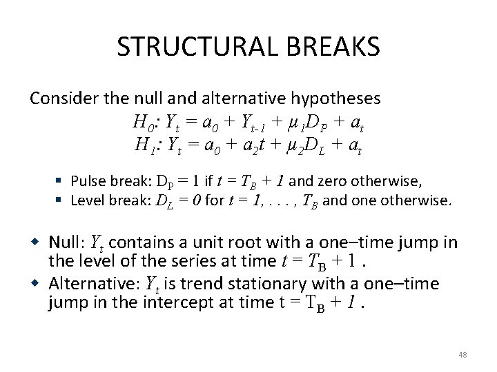
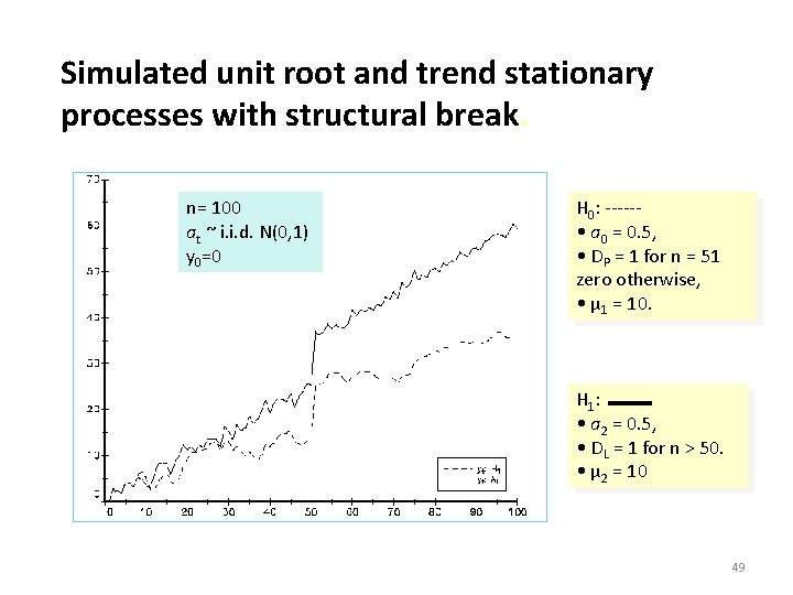
STRUCTURAL BREAKS Consider the null and alternative hypotheses H 0: Yt = a 0 + Yt-1 + µ 1 DP + at H 1: Yt = a 0 + a 2 t + µ 2 DL + at § Pulse break: DP = 1 if t = TB + 1 and zero otherwise, § Level break: DL = 0 for t = 1, . . . , TB and one otherwise. w Null: Yt contains a unit root with a one–time jump in the level of the series at time t = TB + 1. w Alternative: Yt is trend stationary with a one–time jump in the intercept at time t = TB + 1. 48

Simulated unit root and trend stationary processes with structural break. n= 100 at ~ i. i. d. N(0, 1) y 0=0 H 0: ----- • a 0 = 0. 5, • DP = 1 for n = 51 zero otherwise, • µ 1 = 10. H 1: • a 2 = 0. 5, • DL = 1 for n > 50. • µ 2 = 10 49

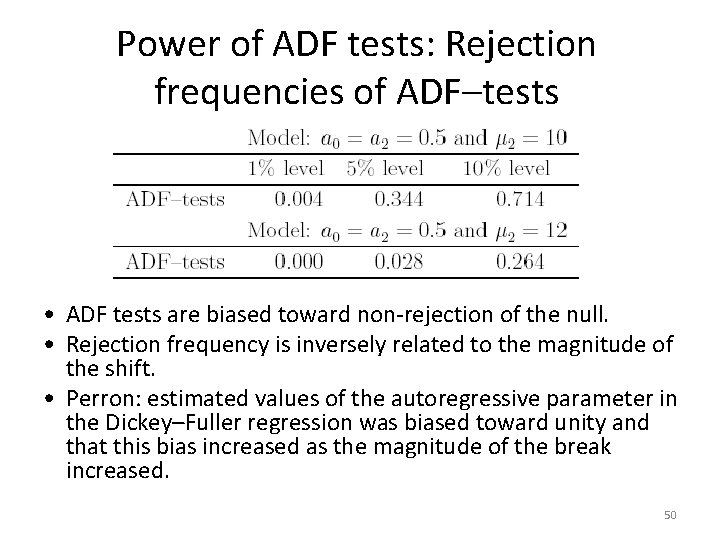
Power of ADF tests: Rejection frequencies of ADF–tests • ADF tests are biased toward non-rejection of the null. • Rejection frequency is inversely related to the magnitude of the shift. • Perron: estimated values of the autoregressive parameter in the Dickey–Fuller regression was biased toward unity and that this bias increased as the magnitude of the break increased. 50

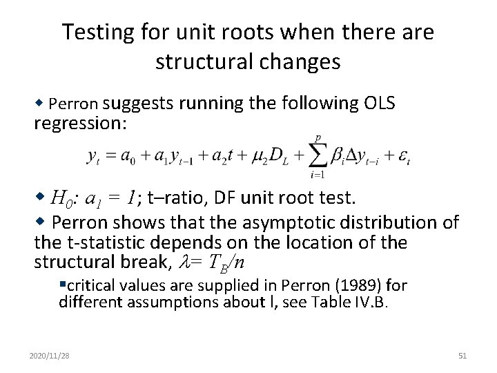
Testing for unit roots when there are structural changes w Perron suggests running the following OLS regression: w H 0: a 1 = 1; t–ratio, DF unit root test. w Perron shows that the asymptotic distribution of the t-statistic depends on the location of the structural break, = TB/n §critical values are supplied in Perron (1989) for different assumptions about l, see Table IV. B. 2020/11/28 51

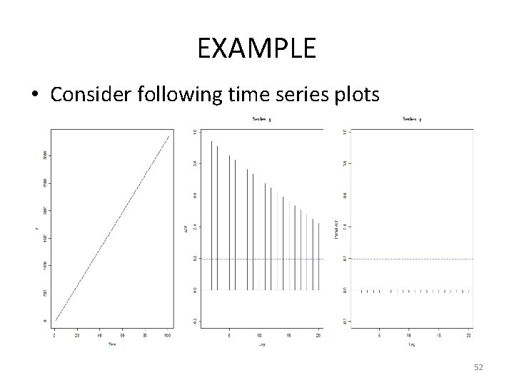
EXAMPLE • Consider following time series plots 52

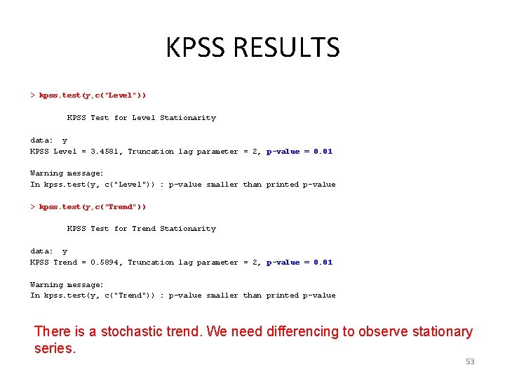
KPSS RESULTS > kpss. test(y, c("Level")) KPSS Test for Level Stationarity data: y KPSS Level = 3. 4581, Truncation lag parameter = 2, p-value = 0. 01 Warning message: In kpss. test(y, c("Level")) : p-value smaller than printed p-value > kpss. test(y, c("Trend")) KPSS Test for Trend Stationarity data: y KPSS Trend = 0. 5894, Truncation lag parameter = 2, p-value = 0. 01 Warning message: In kpss. test(y, c("Trend")) : p-value smaller than printed p-value There is a stochastic trend. We need differencing to observe stationary series. 53

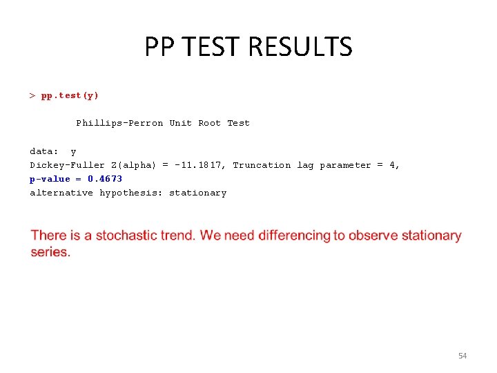
PP TEST RESULTS > pp. test(y) Phillips-Perron Unit Root Test data: y Dickey-Fuller Z(alpha) = -11. 1817, Truncation lag parameter = 4, p-value = 0. 4673 alternative hypothesis: stationary 54

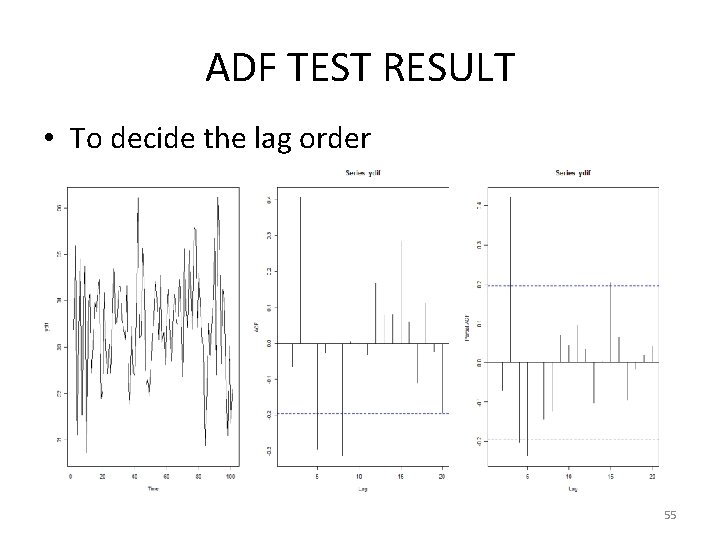
ADF TEST RESULT • To decide the lag order 55

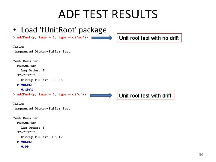
ADF TEST RESULTS • Load ‘f. Unit. Root’ package > adf. Test(y, lags = 5, type = c("nc")) Unit root test with no drift Title: Augmented Dickey-Fuller Test Results: PARAMETER: Lag Order: 5 STATISTIC: Dickey-Fuller: -0. 3663 P VALUE: 0. 4964 > adf. Test(y, lags = 5, type = c("c")) Unit root test with drift Title: Augmented Dickey-Fuller Test Results: PARAMETER: Lag Order: 5 STATISTIC: Dickey-Fuller: 0. 6517 P VALUE: 0. 99 56

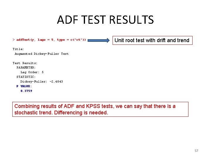
ADF TEST RESULTS > adf. Test(y, lags = 5, type = c("ct")) Unit root test with drift and trend Title: Augmented Dickey-Fuller Test Results: PARAMETER: Lag Order: 5 STATISTIC: Dickey-Fuller: -2. 4843 P VALUE: 0. 3759 Combining results of ADF and KPSS tests, we can say that there is a stochastic trend. Differencing is needed. 57

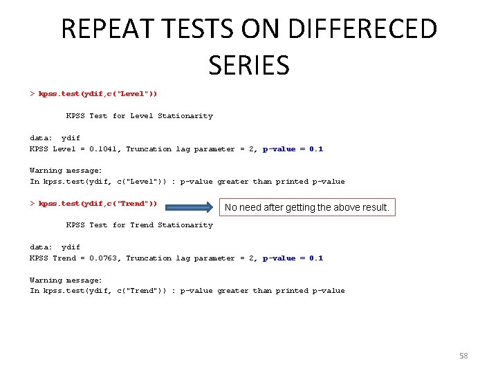
REPEAT TESTS ON DIFFERECED SERIES > kpss. test(ydif, c("Level")) KPSS Test for Level Stationarity data: ydif KPSS Level = 0. 1041, Truncation lag parameter = 2, p-value = 0. 1 Warning message: In kpss. test(ydif, c("Level")) : p-value greater than printed p-value > kpss. test(ydif, c("Trend")) No need after getting the above result. KPSS Test for Trend Stationarity data: ydif KPSS Trend = 0. 0763, Truncation lag parameter = 2, p-value = 0. 1 Warning message: In kpss. test(ydif, c("Trend")) : p-value greater than printed p-value 58

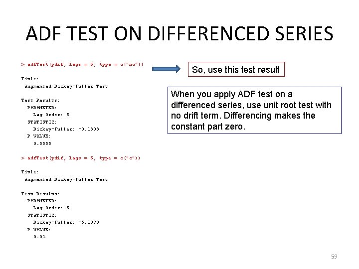
ADF TEST ON DIFFERENCED SERIES > adf. Test(ydif, lags = 5, type = c("nc")) So, use this test result Title: Augmented Dickey-Fuller Test Results: PARAMETER: Lag Order: 5 STATISTIC: Dickey-Fuller: -0. 1808 P VALUE: 0. 5555 When you apply ADF test on a differenced series, use unit root test with no drift term. Differencing makes the constant part zero. > adf. Test(ydif, lags = 5, type = c("c")) Title: Augmented Dickey-Fuller Test Results: PARAMETER: Lag Order: 5 STATISTIC: Dickey-Fuller: -5. 1038 P VALUE: 0. 01 59

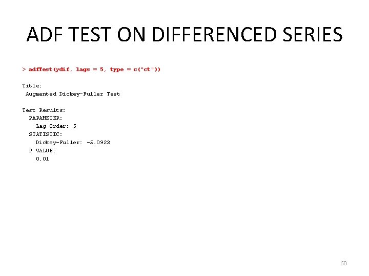
ADF TEST ON DIFFERENCED SERIES > adf. Test(ydif, lags = 5, type = c("ct")) Title: Augmented Dickey-Fuller Test Results: PARAMETER: Lag Order: 5 STATISTIC: Dickey-Fuller: -5. 0923 P VALUE: 0. 01 60

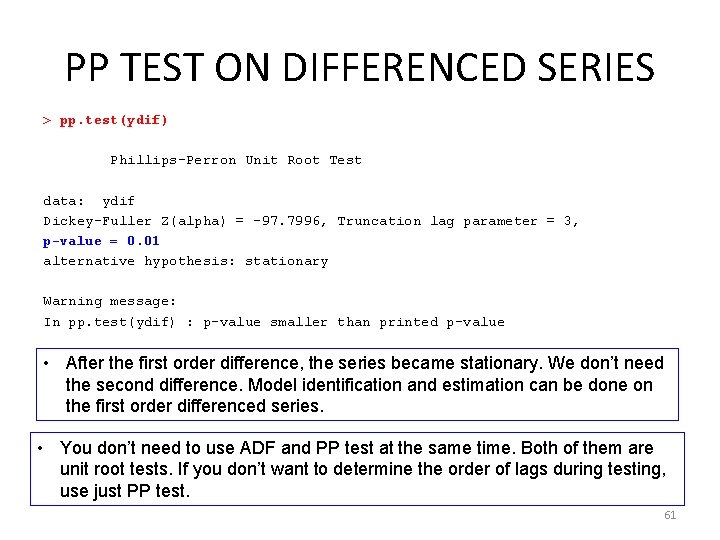
PP TEST ON DIFFERENCED SERIES > pp. test(ydif) Phillips-Perron Unit Root Test data: ydif Dickey-Fuller Z(alpha) = -97. 7996, Truncation lag parameter = 3, p-value = 0. 01 alternative hypothesis: stationary Warning message: In pp. test(ydif) : p-value smaller than printed p-value • After the first order difference, the series became stationary. We don’t need the second difference. Model identification and estimation can be done on the first order differenced series. • You don’t need to use ADF and PP test at the same time. Both of them are unit root tests. If you don’t want to determine the order of lags during testing, use just PP test. 61