Chapter 17 LeastSquares Regression Lecture Notes Dr Rakhmad

Chapter 17 Least-Squares Regression Lecture Notes Dr. Rakhmad Arief Siregar Universiti Malaysia Perlis Applied Numerical Method for Engineers 1

2

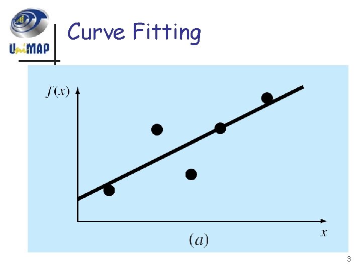
Curve Fitting 3

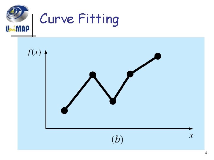
Curve Fitting 4

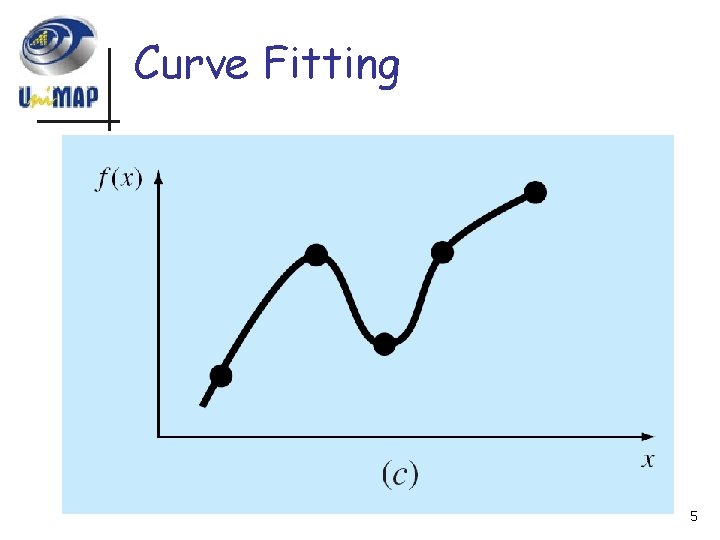
Curve Fitting 5

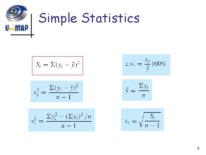
Simple Statistics 6

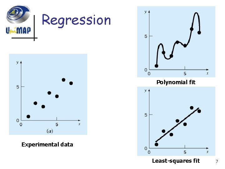
Regression Polynomial fit Experimental data Least-squares fit 7

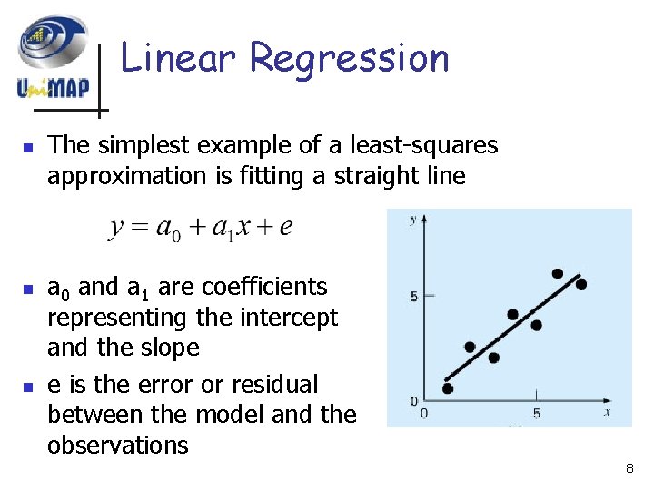
Linear Regression n The simplest example of a least-squares approximation is fitting a straight line a 0 and a 1 are coefficients representing the intercept and the slope e is the error or residual between the model and the observations 8

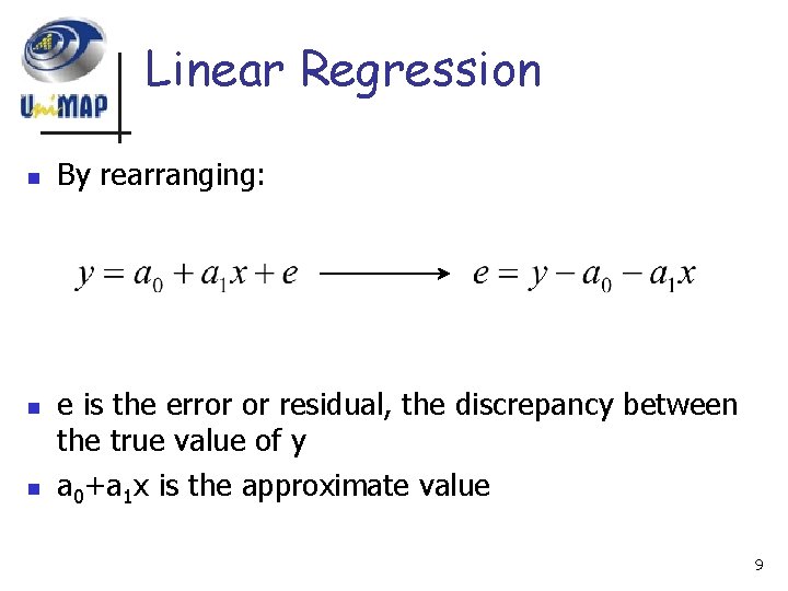
Linear Regression n By rearranging: e is the error or residual, the discrepancy between the true value of y a 0+a 1 x is the approximate value 9

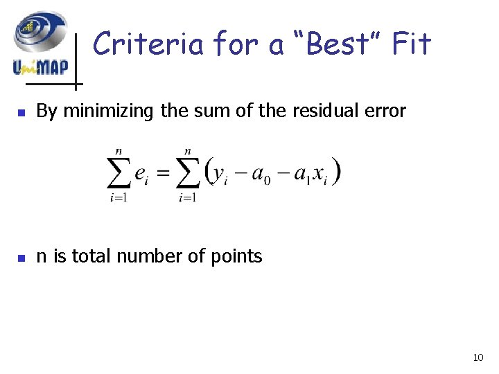
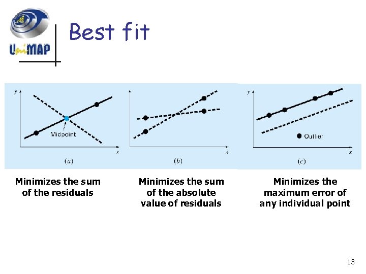
Criteria for a “Best” Fit n By minimizing the sum of the residual error n n is total number of points 10

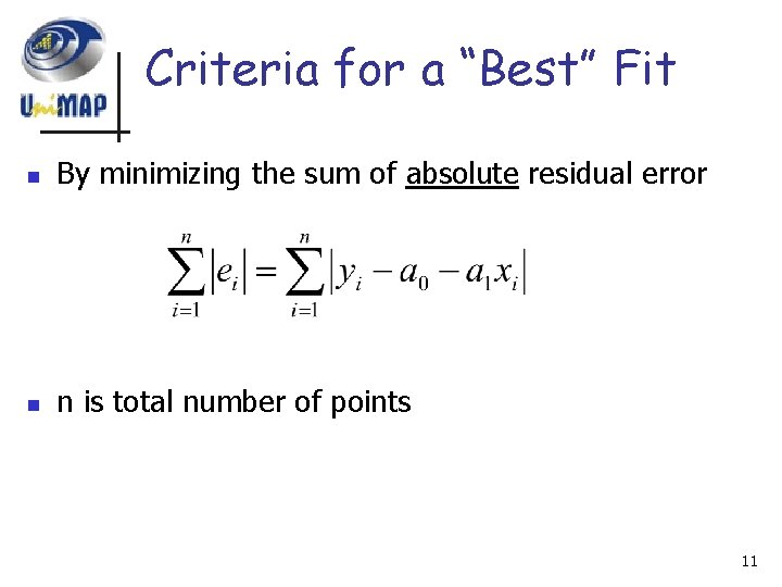
Criteria for a “Best” Fit n By minimizing the sum of absolute residual error n n is total number of points 11

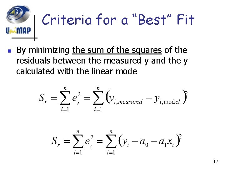
Criteria for a “Best” Fit n By minimizing the sum of the squares of the residuals between the measured y and the y calculated with the linear mode 12

Best fit Minimizes the sum of the residuals Minimizes the sum of the absolute value of residuals Minimizes the maximum error of any individual point 13

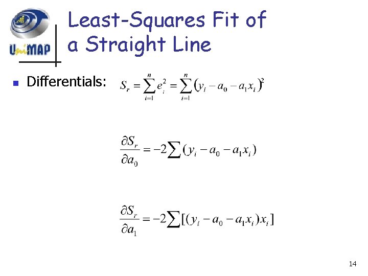
Least-Squares Fit of a Straight Line n Differentials: 14

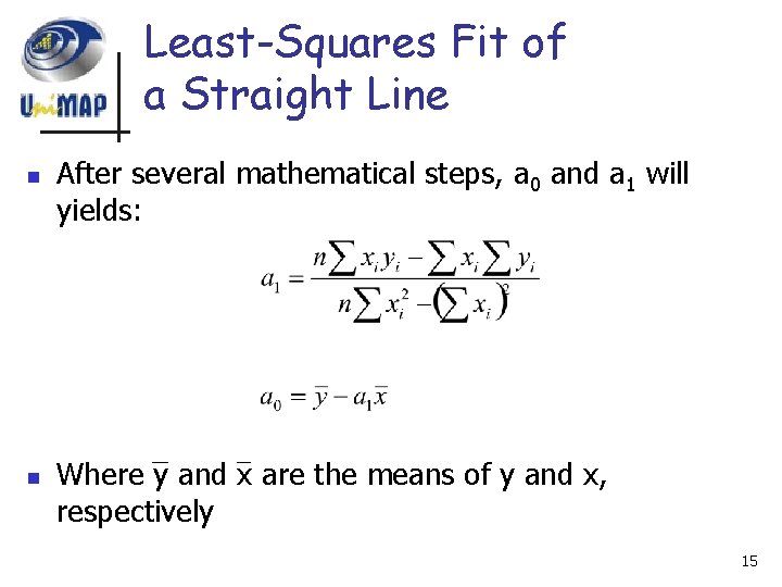
Least-Squares Fit of a Straight Line n n After several mathematical steps, a 0 and a 1 will yields: Where y and x are the means of y and x, respectively 15

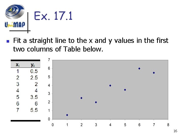
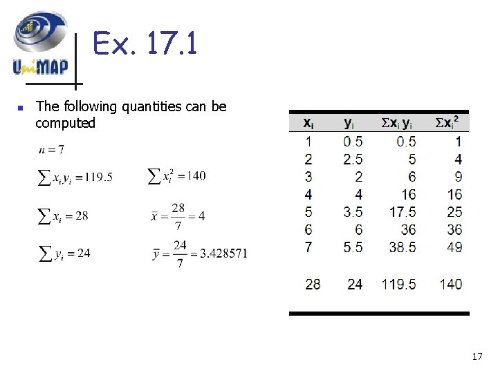
Ex. 17. 1 n Fit a straight line to the x and y values in the first two columns of Table below. 16

Ex. 17. 1 n The following quantities can be computed 17

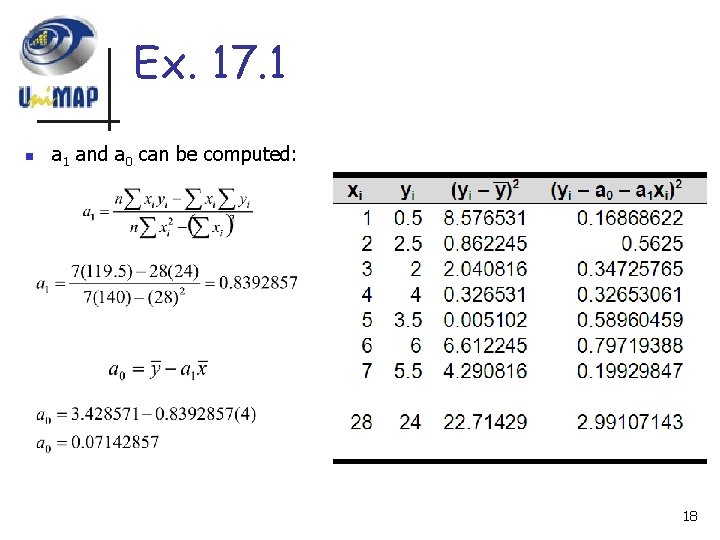
Ex. 17. 1 n a 1 and a 0 can be computed: 18

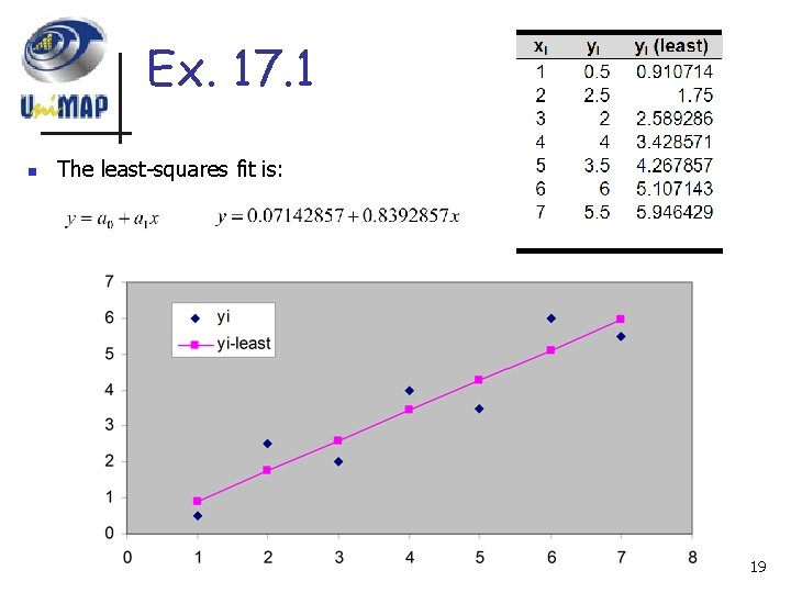
Ex. 17. 1 n The least-squares fit is: 19

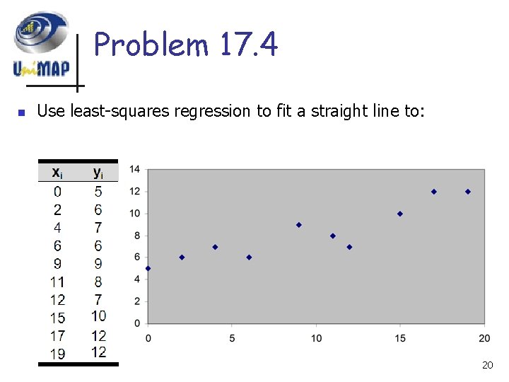
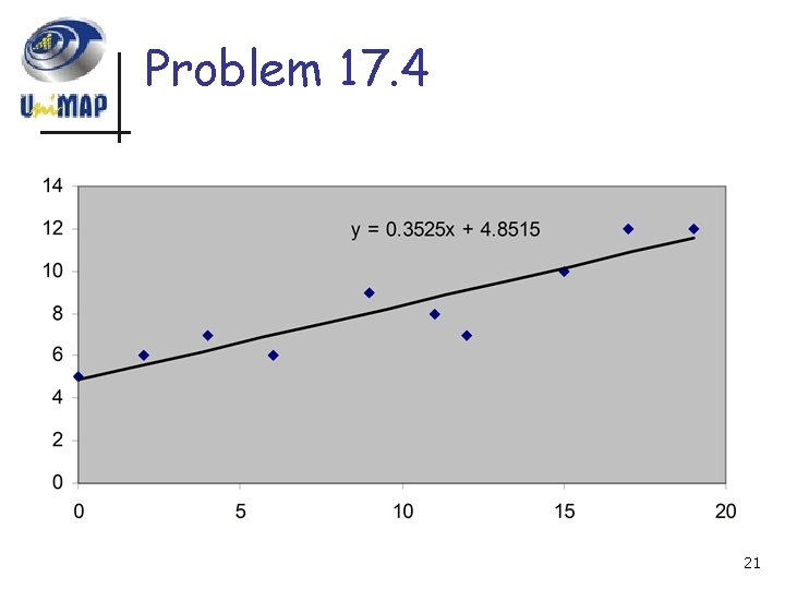
Problem 17. 4 n Use least-squares regression to fit a straight line to: 20

Problem 17. 4 21

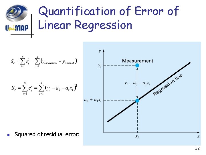
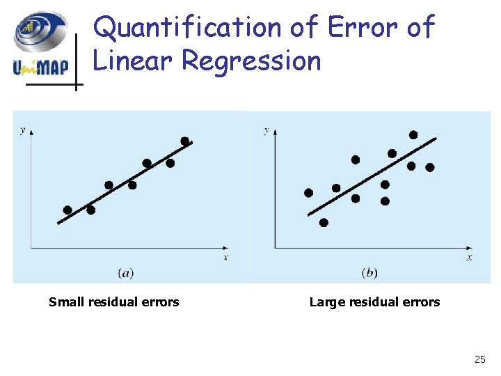
Quantification of Error of Linear Regression n Squared of residual error: 22

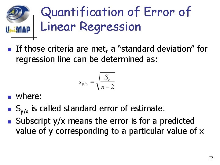
Quantification of Error of Linear Regression n n If those criteria are met, a “standard deviation” for regression line can be determined as: where: Sy/x is called standard error of estimate. Subscript y/x means the error is for a predicted value of y corresponding to a particular value of x 23

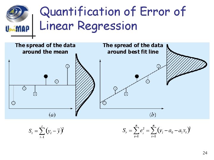
Quantification of Error of Linear Regression The spread of the data around the mean The spread of the data around best fit line 24

Quantification of Error of Linear Regression Small residual errors Large residual errors 25

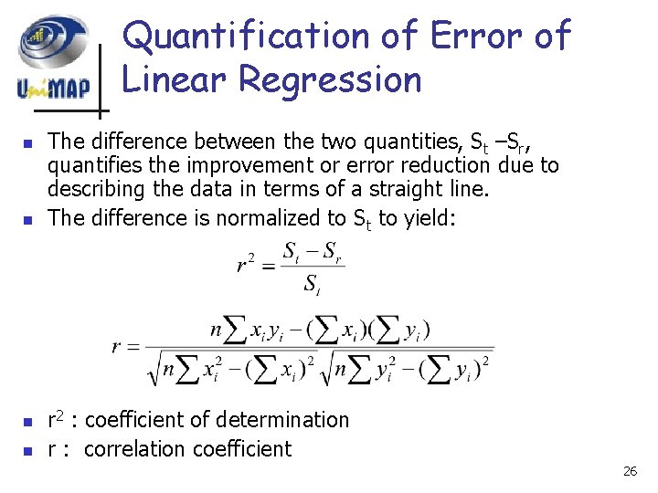
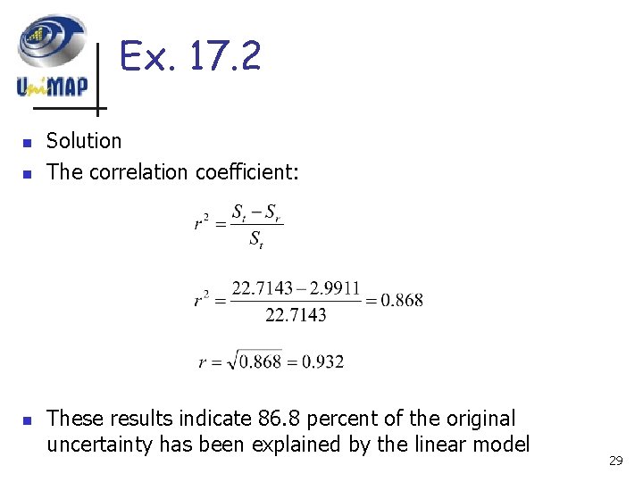
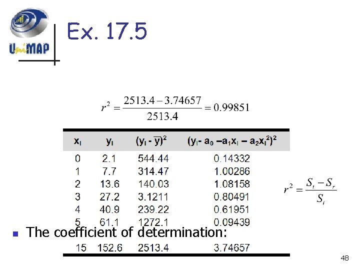
Quantification of Error of Linear Regression n n The difference between the two quantities, St –Sr, quantifies the improvement or error reduction due to describing the data in terms of a straight line. The difference is normalized to St to yield: r 2 : coefficient of determination r : correlation coefficient 26

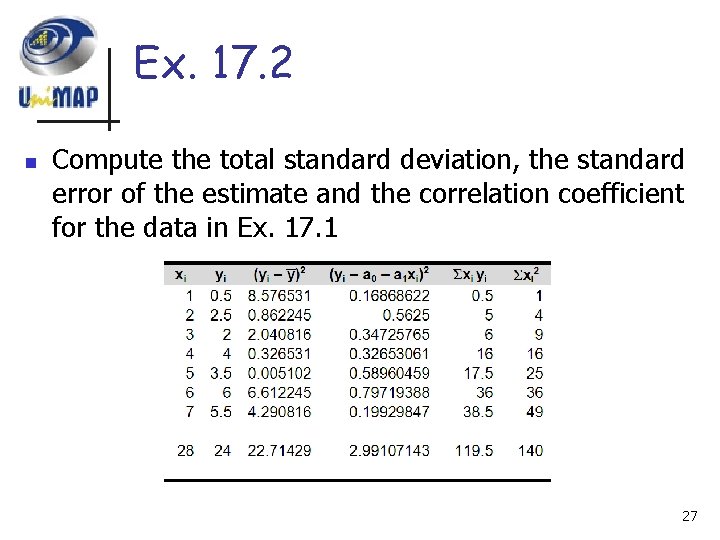
Ex. 17. 2 n Compute the total standard deviation, the standard error of the estimate and the correlation coefficient for the data in Ex. 17. 1 27

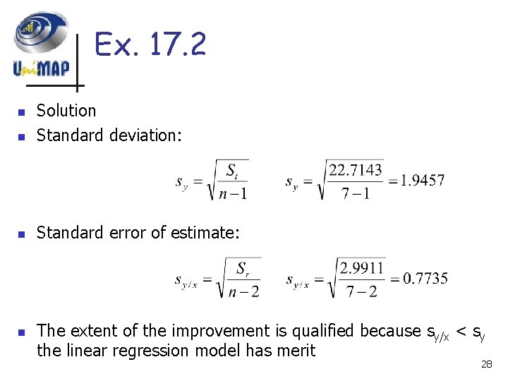
Ex. 17. 2 n Solution Standard deviation: n Standard error of estimate: n n The extent of the improvement is qualified because sy/x < sy the linear regression model has merit 28

Ex. 17. 2 n n n Solution The correlation coefficient: These results indicate 86. 8 percent of the original uncertainty has been explained by the linear model 29

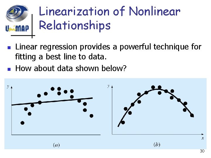
Linearization of Nonlinear Relationships n n Linear regression provides a powerful technique for fitting a best line to data. How about data shown below? 30

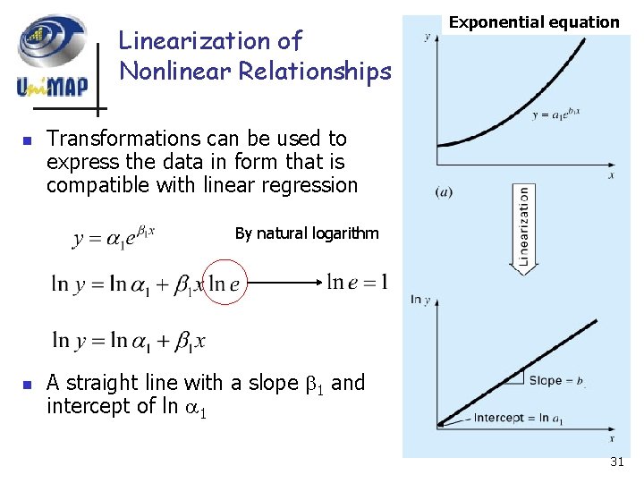
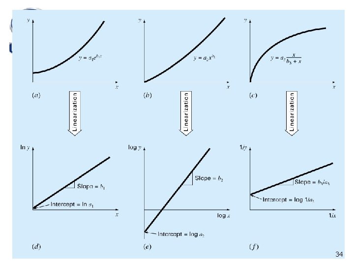
Linearization of Nonlinear Relationships n Exponential equation Transformations can be used to express the data in form that is compatible with linear regression By natural logarithm n A straight line with a slope 1 and intercept of ln 1 31

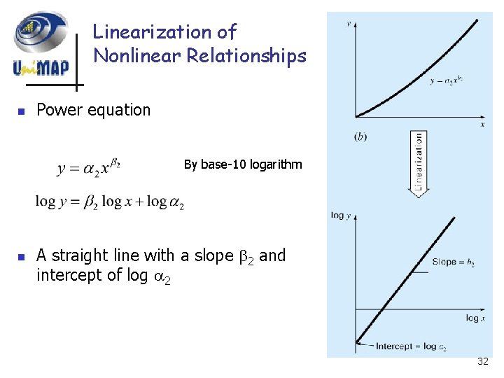
Linearization of Nonlinear Relationships n Power equation By base-10 logarithm n A straight line with a slope 2 and intercept of log 2 32

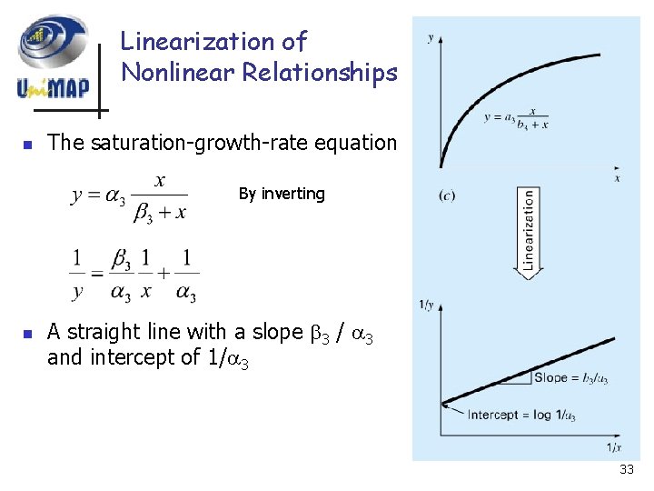
Linearization of Nonlinear Relationships n The saturation-growth-rate equation By inverting n A straight line with a slope 3 / 3 and intercept of 1/ 3 33

34

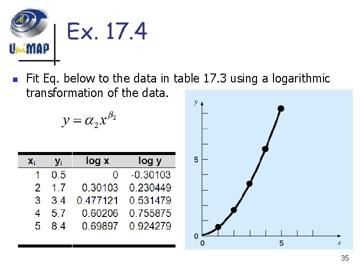
Ex. 17. 4 n Fit Eq. below to the data in table 17. 3 using a logarithmic transformation of the data. 35

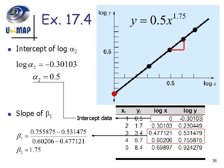
Ex. 17. 4 n Intercept of log 2 n Slope of 1 Intercept data 36

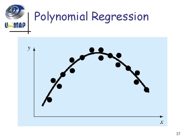
Polynomial Regression 37

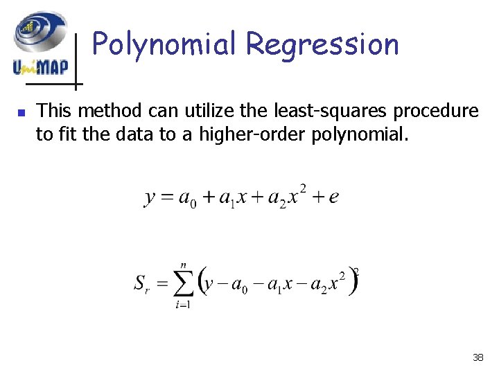
Polynomial Regression n This method can utilize the least-squares procedure to fit the data to a higher-order polynomial. 38

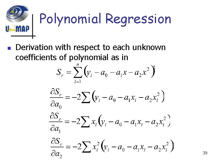
Polynomial Regression n Derivation with respect to each unknown coefficients of polynomial as in 39

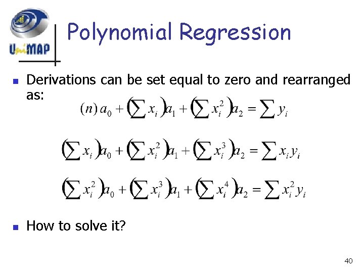
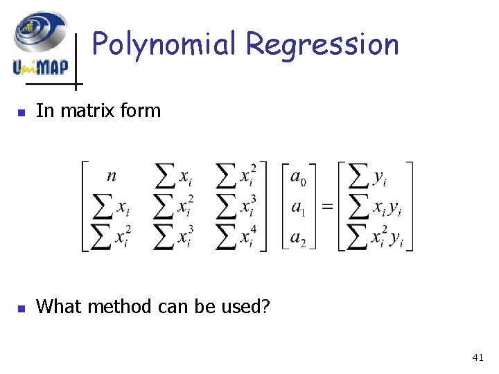
Polynomial Regression n n Derivations can be set equal to zero and rearranged as: How to solve it? 40

Polynomial Regression n In matrix form n What method can be used? 41

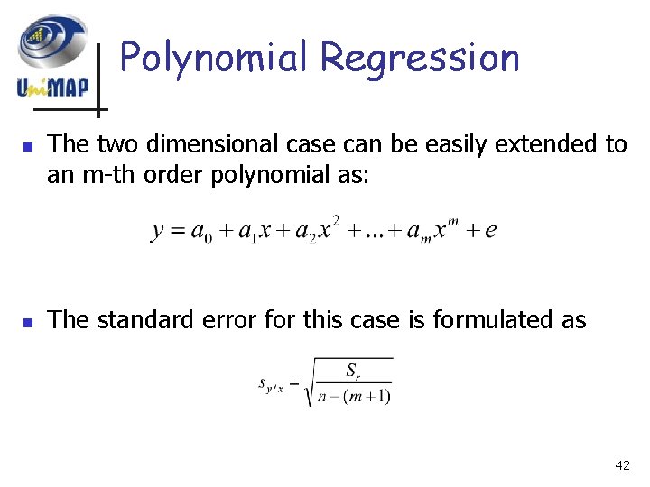
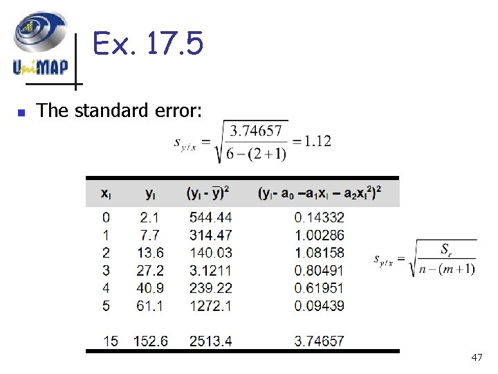
Polynomial Regression n n The two dimensional case can be easily extended to an m-th order polynomial as: The standard error for this case is formulated as 42

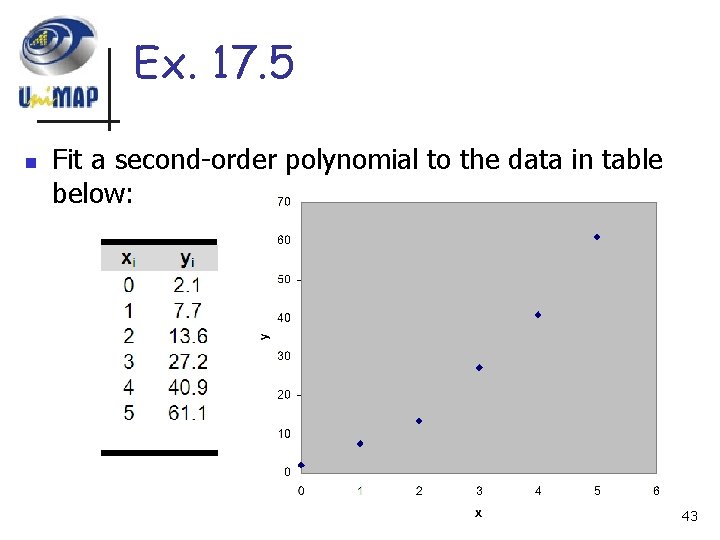
Ex. 17. 5 n Fit a second-order polynomial to the data in table below: 43

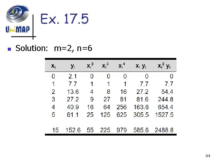
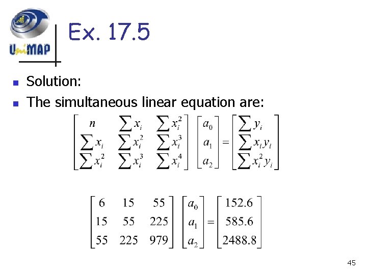
Ex. 17. 5 n Solution: m=2, n=6 44

Ex. 17. 5 n n Solution: The simultaneous linear equation are: 45

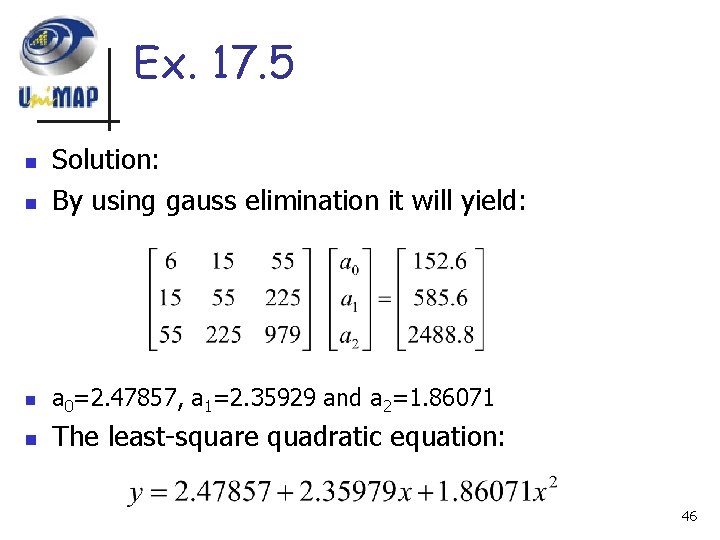
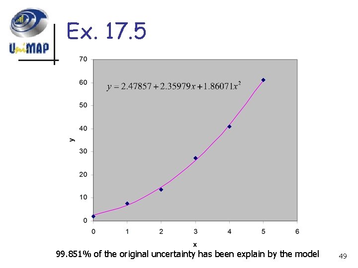
Ex. 17. 5 n Solution: By using gauss elimination it will yield: n a 0=2. 47857, a 1=2. 35929 and a 2=1. 86071 n The least-square quadratic equation: n 46

Ex. 17. 5 n The standard error: 47

Ex. 17. 5 n The coefficient of determination: 48

Ex. 17. 5 99. 851% of the original uncertainty has been explain by the model 49

Assignment 3 n n Do Problems 17. 5, 17. 6, 17. 7, 17. 10 and 17. 12 Submit next week 50

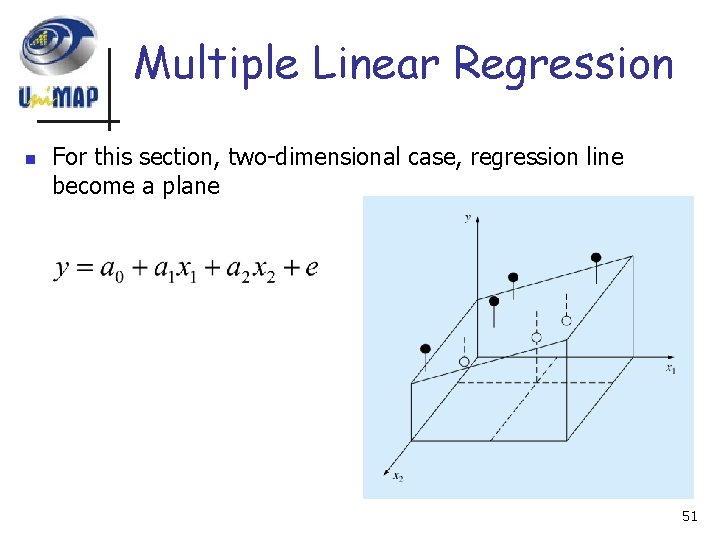
Multiple Linear Regression n For this section, two-dimensional case, regression line become a plane 51

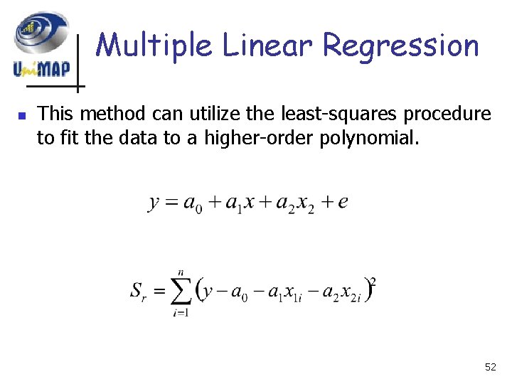
Multiple Linear Regression n This method can utilize the least-squares procedure to fit the data to a higher-order polynomial. 52

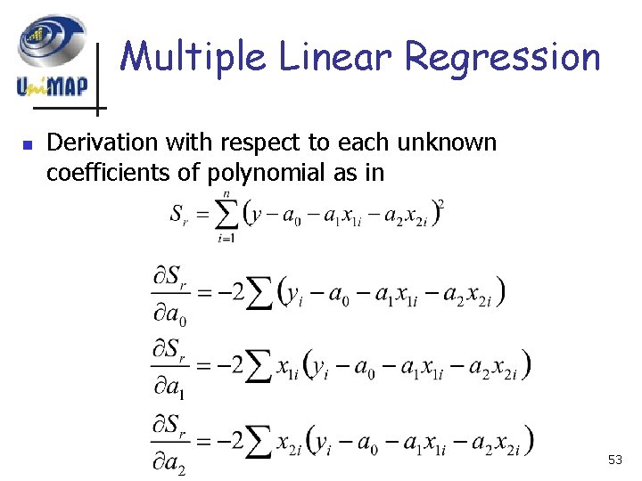
Multiple Linear Regression n Derivation with respect to each unknown coefficients of polynomial as in 53

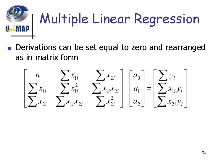
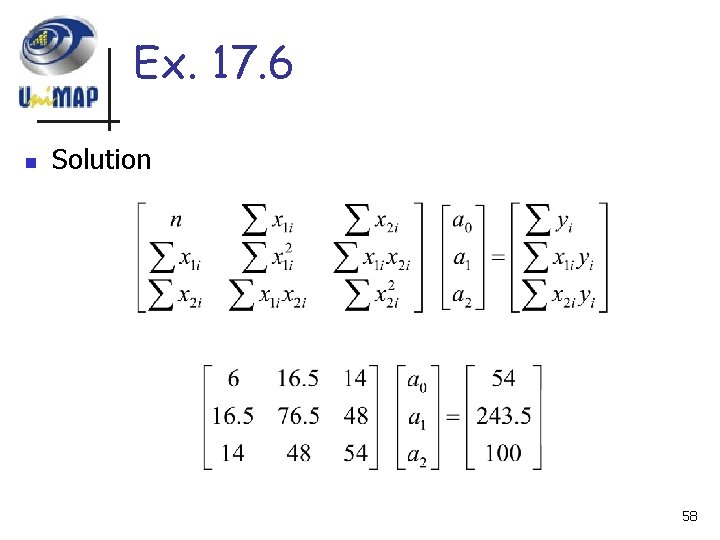
Multiple Linear Regression n Derivations can be set equal to zero and rearranged as in matrix form 54

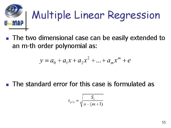
Multiple Linear Regression n n The two dimensional case can be easily extended to an m-th order polynomial as: The standard error for this case is formulated as 55

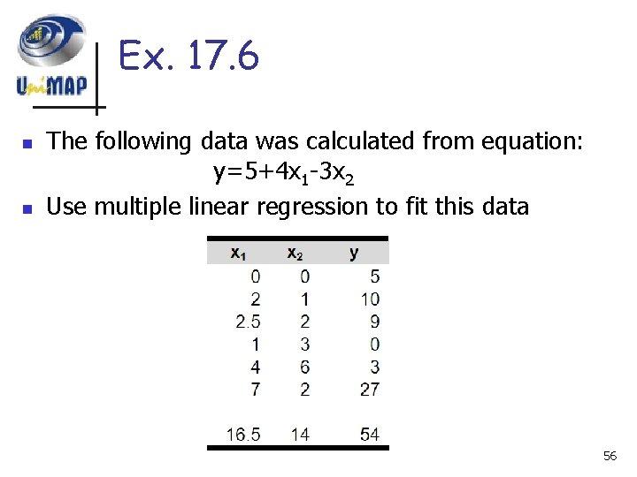
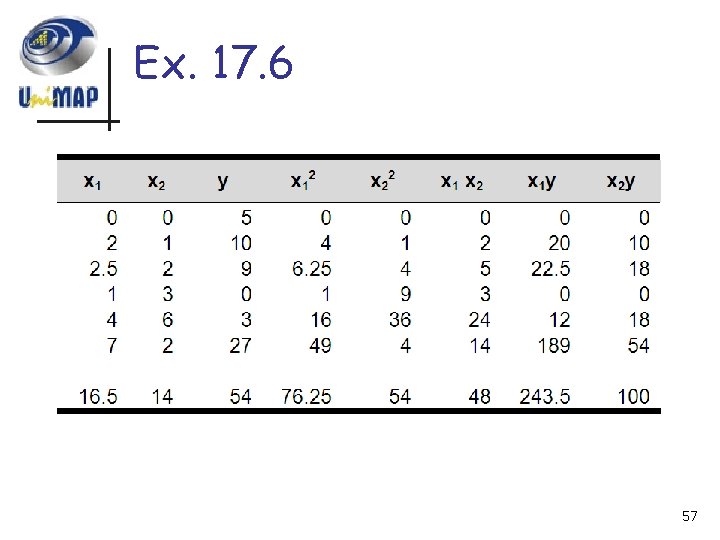
Ex. 17. 6 n n The following data was calculated from equation: y=5+4 x 1 -3 x 2 Use multiple linear regression to fit this data 56

Ex. 17. 6 57

Ex. 17. 6 n Solution 58

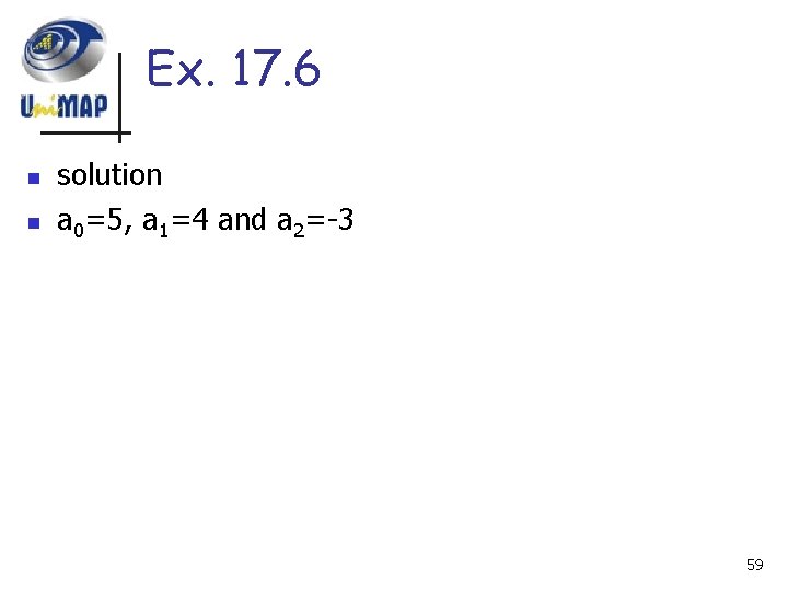
Ex. 17. 6 n n solution a 0=5, a 1=4 and a 2=-3 59

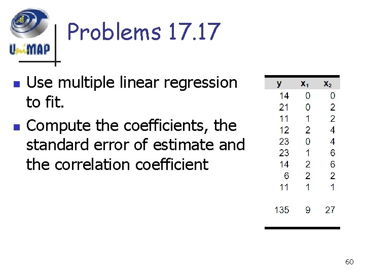
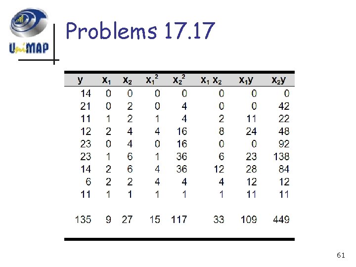
Problems 17. 17 n n Use multiple linear regression to fit. Compute the coefficients, the standard error of estimate and the correlation coefficient 60

Problems 17. 17 61

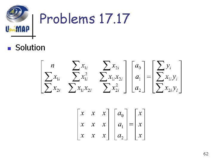
Problems 17. 17 n Solution 62

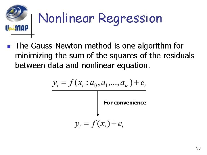
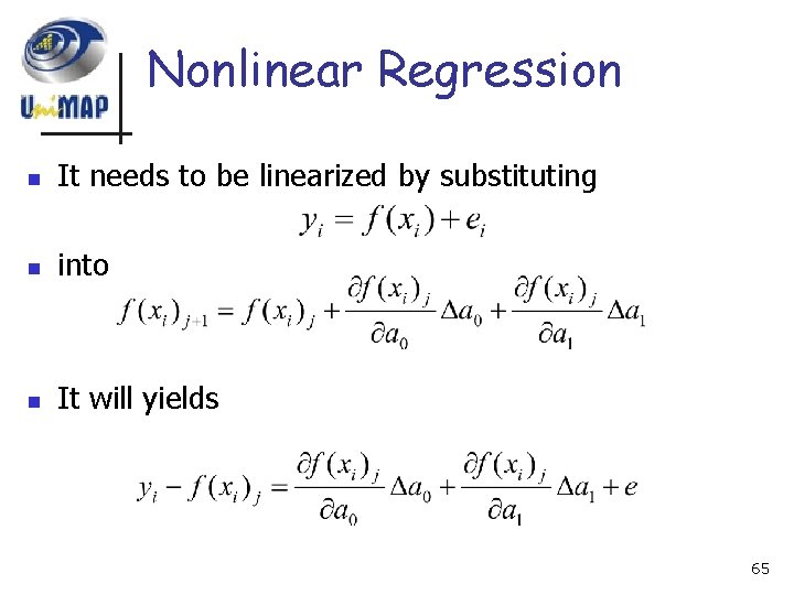
Nonlinear Regression n The Gauss-Newton method is one algorithm for minimizing the sum of the squares of the residuals between data and nonlinear equation. For convenience 63

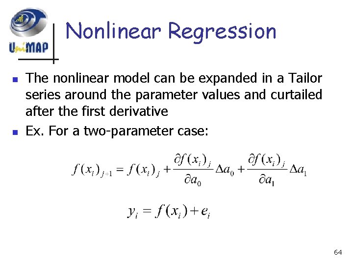
Nonlinear Regression n n The nonlinear model can be expanded in a Tailor series around the parameter values and curtailed after the first derivative Ex. For a two-parameter case: 64

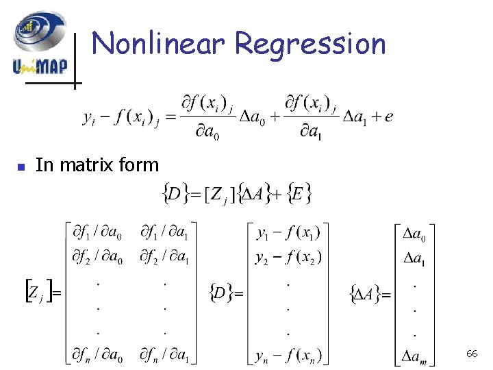
Nonlinear Regression n It needs to be linearized by substituting n into n It will yields 65

Nonlinear Regression n In matrix form 66

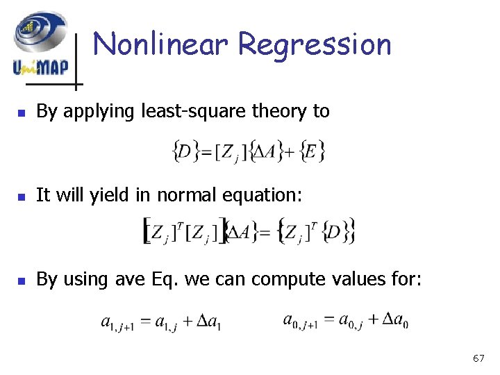
Nonlinear Regression n By applying least-square theory to n It will yield in normal equation: n By using ave Eq. we can compute values for: 67

Ex. 17. 9 68