LEASTSQUARES REGRESSION 3 2 Least Squares Regression Line

LEAST-SQUARES REGRESSION 3. 2 Least Squares Regression Line and Residuals

Recall from 3. 1: Correlation measures the strength and direction of a linear relationship between two variables. How do we summarize the overall pattern of a linear relationship? Draw a line!

Regression Line A regression line summarizes the relationship between two variables, but only in settings where one of the variables helps explain or predict the other.

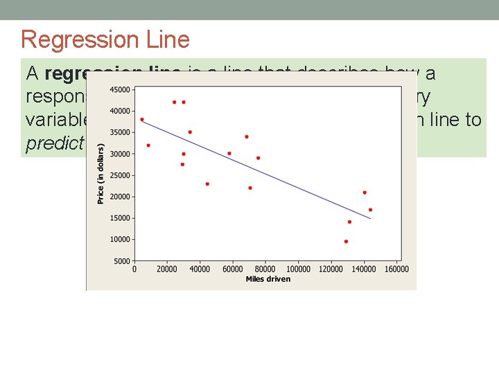
Regression Line A regression line is a line that describes how a response variable y changes as an explanatory variable x changes. We often use a regression line to predict the value of y for a given value of x.

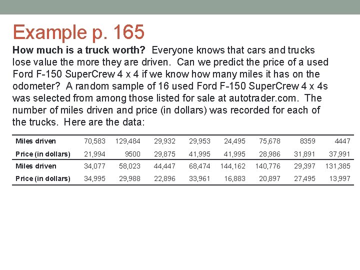
Example p. 165 How much is a truck worth? Everyone knows that cars and trucks lose value the more they are driven. Can we predict the price of a used Ford F-150 Super. Crew 4 x 4 if we know how many miles it has on the odometer? A random sample of 16 used Ford F-150 Super. Crew 4 x 4 s was selected from among those listed for sale at autotrader. com. The number of miles driven and price (in dollars) was recorded for each of the trucks. Here are the data: Miles driven 70, 583 129, 484 29, 932 29, 953 24, 495 75, 678 8359 4447 Price (in dollars) 21, 994 9500 29, 875 41, 995 28, 986 31, 891 37, 991 Miles driven 34, 077 58, 023 44, 447 68, 474 144, 162 140, 776 29, 397 131, 385 Price (in dollars) 34, 995 29, 988 22, 896 33, 961 16, 883 20, 897 27, 495 13, 997

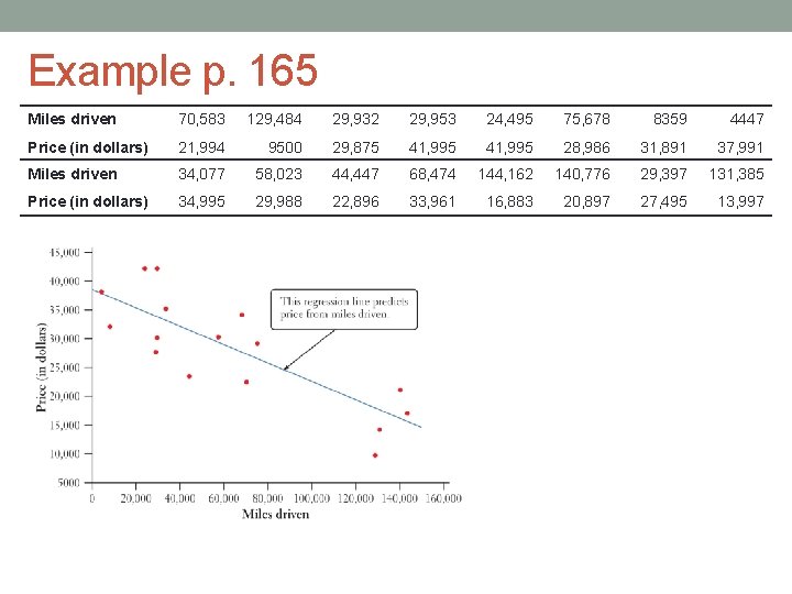
Example p. 165 Miles driven 70, 583 129, 484 29, 932 29, 953 24, 495 75, 678 8359 4447 Price (in dollars) 21, 994 9500 29, 875 41, 995 28, 986 31, 891 37, 991 Miles driven 34, 077 58, 023 44, 447 68, 474 144, 162 140, 776 29, 397 131, 385 Price (in dollars) 34, 995 29, 988 22, 896 33, 961 16, 883 20, 897 27, 495 13, 997

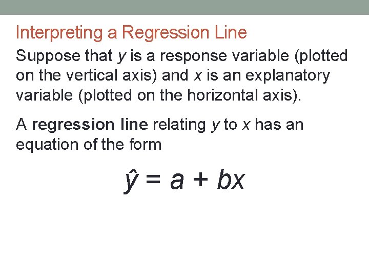
Interpreting a Regression Line Suppose that y is a response variable (plotted on the vertical axis) and x is an explanatory variable (plotted on the horizontal axis). A regression line relating y to x has an equation of the form ŷ = a + bx

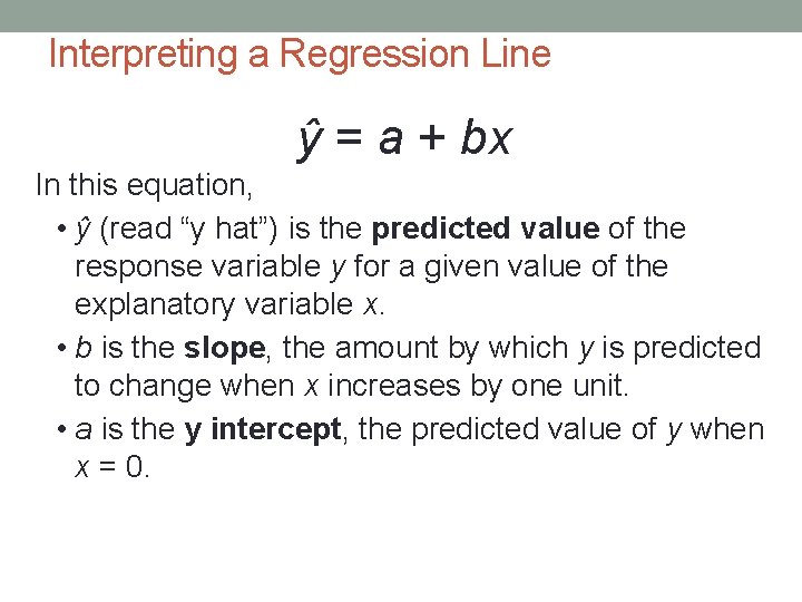
Interpreting a Regression Line ŷ = a + bx In this equation, • ŷ (read “y hat”) is the predicted value of the response variable y for a given value of the explanatory variable x. • b is the slope, the amount by which y is predicted to change when x increases by one unit. • a is the y intercept, the predicted value of y when x = 0.

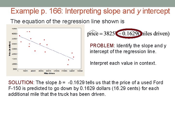
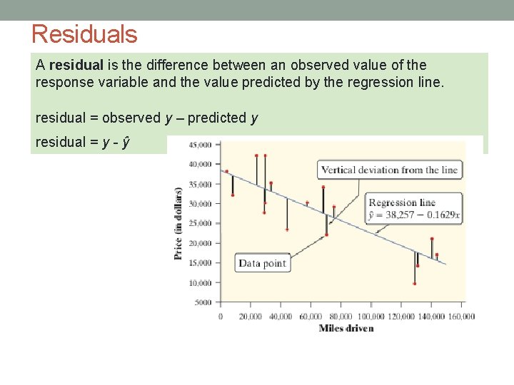
Example p. 166: Interpreting slope and y intercept The equation of the regression line shown is PROBLEM: Identify the slope and y intercept of the regression line. Interpret each value in context. SOLUTION: The slope b = -0. 1629 tells us that the price of a used Ford F-150 is predicted to go down by 0. 1629 dollars (16. 29 cents) for each additional mile that the truck has been driven.

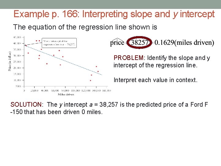
Example p. 166: Interpreting slope and y intercept The equation of the regression line shown is PROBLEM: Identify the slope and y intercept of the regression line. Interpret each value in context. SOLUTION: The y intercept a = 38, 257 is the predicted price of a Ford F -150 that has been driven 0 miles.

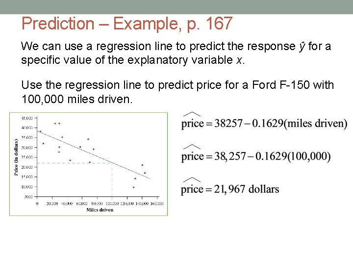
Prediction – Example, p. 167 We can use a regression line to predict the response ŷ for a specific value of the explanatory variable x. Use the regression line to predict price for a Ford F-150 with 100, 000 miles driven.

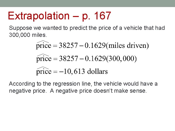
Extrapolation – p. 167 Suppose we wanted to predict the price of a vehicle that had 300, 000 miles. According to the regression line, the vehicle would have a negative price. A negative price doesn’t make sense.

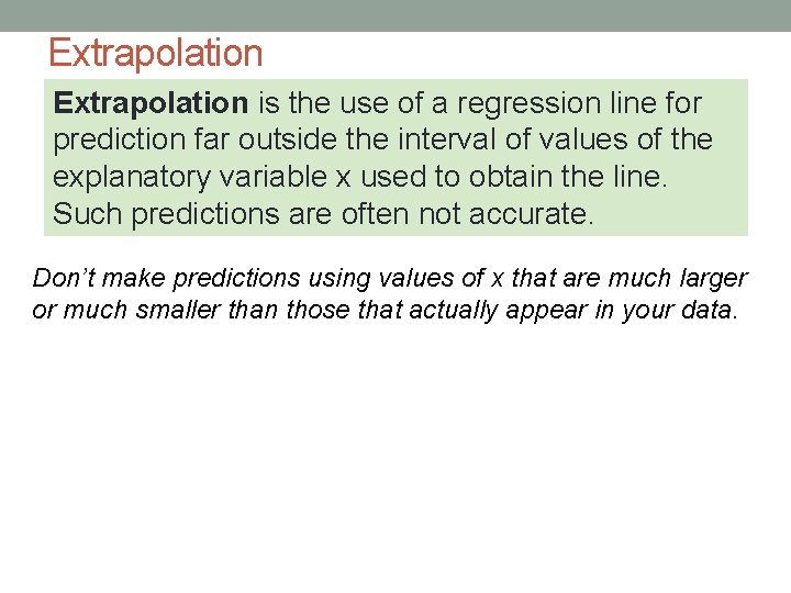
Extrapolation is the use of a regression line for prediction far outside the interval of values of the explanatory variable x used to obtain the line. Such predictions are often not accurate. Don’t make predictions using values of x that are much larger or much smaller than those that actually appear in your data.

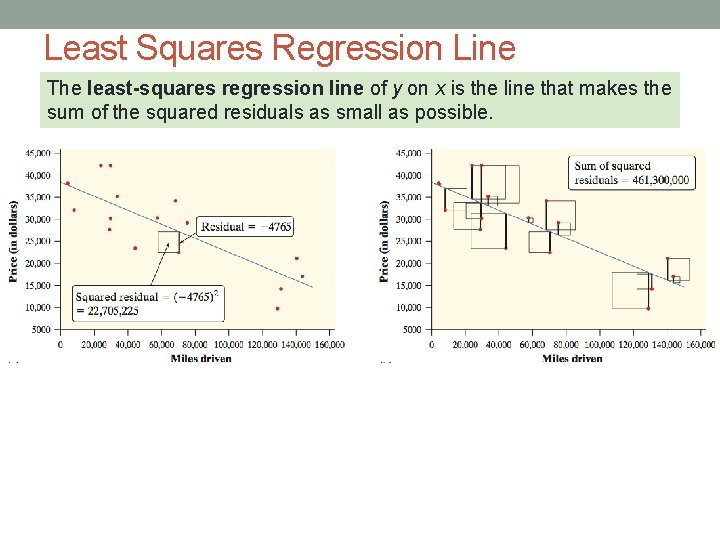
Residuals A residual is the difference between an observed value of the response variable and the value predicted by the regression line. residual = observed y – predicted y residual = y - ŷ

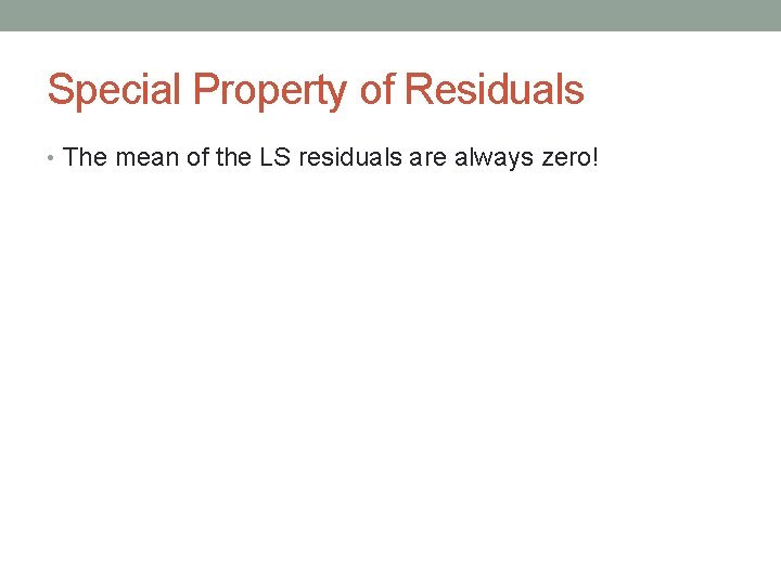
Special Property of Residuals • The mean of the LS residuals are always zero!

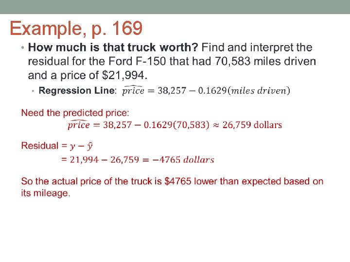
Example, p. 169 •

Least Squares Regression Line The least-squares regression line of y on x is the line that makes the sum of the squared residuals as small as possible.

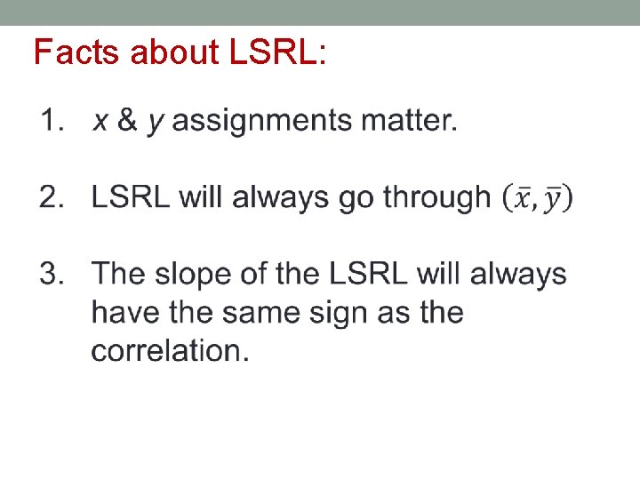
Facts about LSRL:

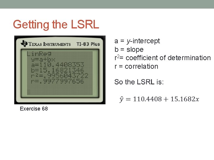
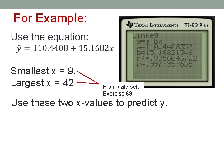
Getting the LSRL a = y-intercept b = slope r 2= coefficient of determination r = correlation Exercise 68

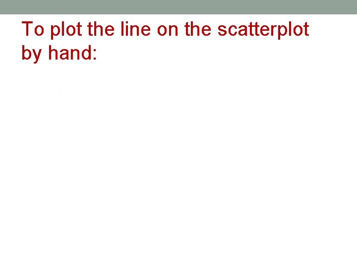
To plot the line on the scatterplot by hand:

For Example: Smallest x = 9, Largest x = 42 From data set: Exercise 68 Use these two x-values to predict y.

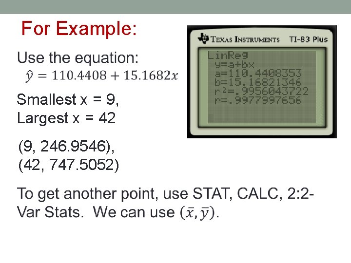
For Example: Smallest x = 9, Largest x = 42 (9, 246. 9546), (42, 747. 5052)

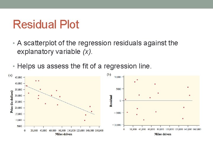
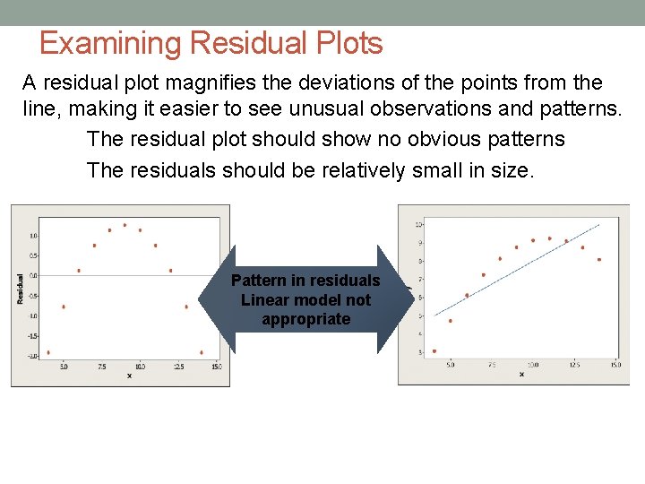
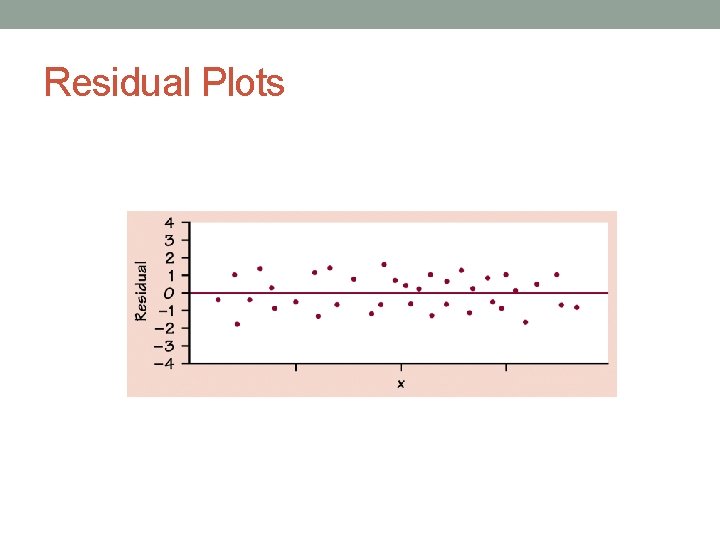
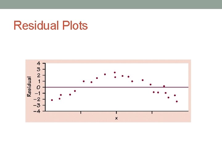
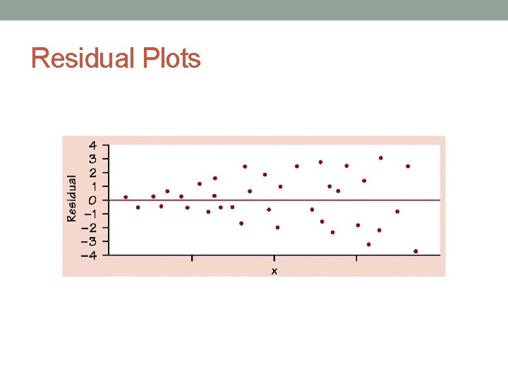
Residual Plot • A scatterplot of the regression residuals against the explanatory variable (x). • Helps us assess the fit of a regression line.

Residuals vs. Correlation • Never rely on correlation alone to determine if an LSRL is the best model for the data. You must check the residual plot!

Examining Residual Plots A residual plot magnifies the deviations of the points from the line, making it easier to see unusual observations and patterns. The residual plot should show no obvious patterns The residuals should be relatively small in size. Pattern in residuals Linear model not appropriate

Residual Plots

Residual Plots

Residual Plots

HW Due: Tuesday • p. 193 & 199 # 35, 39, 41, 45, 52, 54, 76