Bayesian Decision Theory Slides are adapted from Jason

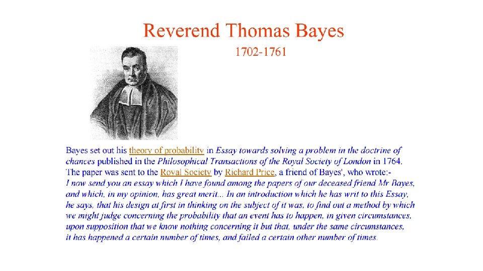
Bayesian Decision Theory Slides are adapted from Jason Corso, George Bebis and Sargur Srihari based on the content from Duda, Hart & Stork

Motivation

Bayesian Decision Theory • Fundamental statistical approach to statistical pattern classification • Quantifies trade-offs between classification using probabilities and costs of decisions • Assumes all relevant probabilities are known

Bayesian Decision Theory It is the decision making when all underlying probability distributions are known. It is optimal given the distributions are known. For two classes w 1 and w 2 , Prior probabilities for an unknown new observation: P(w 1) : the new observation belongs to class 1 P(w 2) : the new observation belongs to class 2 P(w 1 ) + P(w 2 ) = 1 It reflects our prior knowledge. It is our decision rule when no feature on the new object is available: Classify as class 1 if P(w 1 ) > P(w 2 )

Bayesian Decision Theory • Design classifiers to make decisions subject to minimizing an expected ”risk”. • The simplest risk is the classification error (i. e. , assuming that misclassification costs are equal). • When misclassification costs are not equal, the risk can include the cost associated with different misclassifications.

Example

Terminology - consider the sea bass/salmon example • State of nature ω (class label): • e. g. , ω1 for sea bass, ω2 for salmon • Probabilities P(ω1) and P(ω2) (priors): • e. g. , prior knowledge of how likely is to get a sea bass or a salmon • Probability density function p(x) (evidence): • e. g. , how frequently we will measure a pattern with feature value x (e. g. , x corresponds to lightness)

Prior Probability

Prior Probability • The catch of salmon and sea bass is equiprobable • P( 1) = P( 2) (uniform priors) • P( 1) + P( 2) = 1 (exclusivity and exhaustivity) 11

Decision Rule from only Priors Favours the most likely class. or P(error) = min[P(ω1), P(ω2)]

Features and Feature spaces

Class Conditional probability density p(x/ωj) (likelihood) : • The class-conditional probability density function is the probability density function for x, our feature, given that the state of nature is ω • e. g. , how frequently we will measure a pattern with feature value x given that the pattern belongs to class ωj • P(x | 1) and P(x | 2) describe the difference in lightness between populations of sea-bass and salmon

Conditional probability P(ωj /x) (posterior) : • e. g. , the probability that the fish belongs to class ωj given feature x.

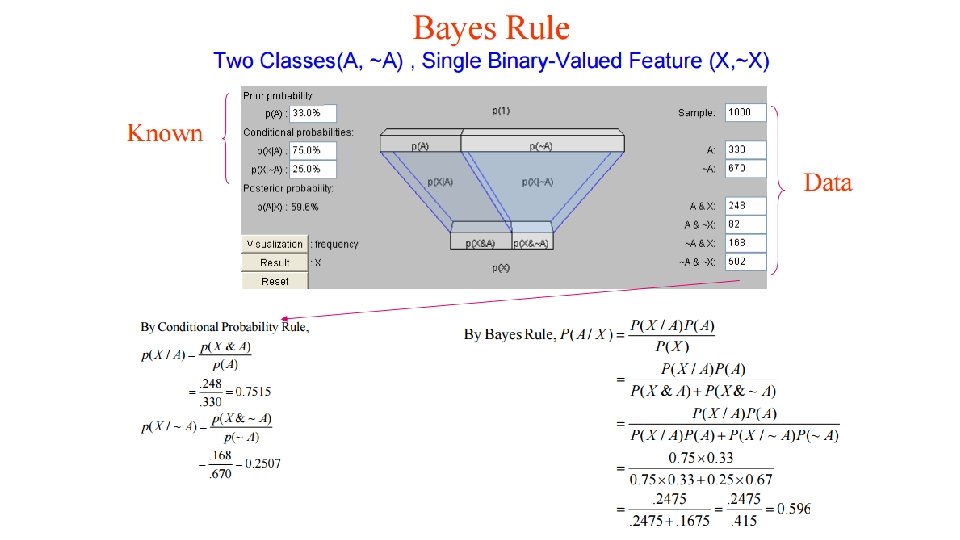
Decision Rule Using Conditional Probabilities • Using Bayes’ rule: where (i. e. , scale factor – sum of probs = 1) Decide ω1 if P(ω1 /x) > P(ω2 /x); otherwise decide ω2 or Decide ω1 if p(x/ω1)P(ω1)>p(x/ω2)P(ω2); otherwise decide ω2 or Decide ω1 if p(x/ω1)/p(x/ω2) >P(ω2)/P(ω1) ; otherwise decide ω2 likelihood ratio threshold

Decision Rule Using Conditional Probabilities (cont’d) p(x/ωj) P(ωj /x)

Probability of error • x is an observation for which: • if P(ω1 | x) > P(ω2 | x) True state of nature = ω1 • if P(ω1 | x) < P(ω2 | x) True state of nature = ω2

Bayes Decision Rule (with equal costs)

Where do Probabilities come from? • There are two competitive answers: (1) Relative frequency (objective) approach. • Probabilities can only come from experiments. (2) Bayesian (subjective) approach. • Probabilities may reflect degree of belief and can be based on opinion.

Example (objective approach) • Classify cars whether they are more or less than $50 K: • Classes: C 1 if price > $50 K, C 2 if price <= $50 K • Features: x, the height of a car • Use the Bayes’ rule to compute the posterior probabilities: • We need to estimate p(x/C 1), p(x/C 2), P(C 1), P(C 2)

Example (cont’d) • Collect data • Ask drivers how much their car was and measure height. • Determine prior probabilities P(C 1), P(C 2) • e. g. , 1209 samples: #C 1=221 #C 2=988

Example (cont’d) • Determine class conditional probabilities (likelihood) • Discretize car height into bins and use normalized histogram

Example (cont’d) • Calculate the posterior probability for each bin:

A More General Theory • Use more than one features. • Allow more than two categories. • Allow actions other than classifying the input to one of the possible categories (e. g. , rejection) - Refusing to make a decision in close or bad cases!. • Employ a more general error function (i. e. , expected “risk”) by associating a “cost” (based on a “loss” function) with different errors. • Note that, the loss function states how costly each action taken is

Loss Function If action i is taken and the true state of nature is j then the decision is correct if i = j and in error if i j Seek a decision rule that minimizes the probability of error which is the error rate

Expected loss

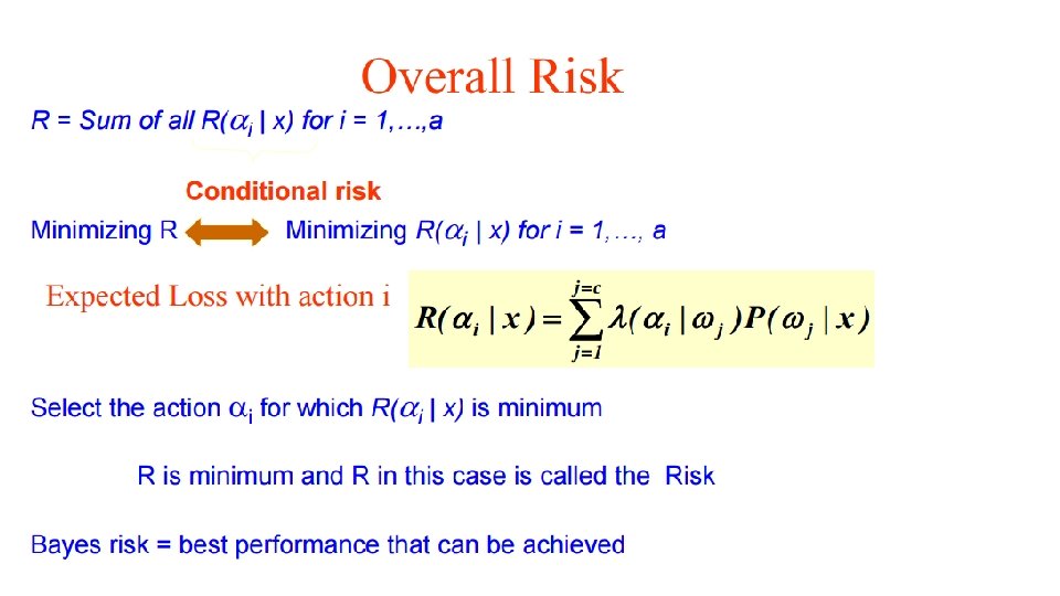
Overall Risk • Suppose α(x) is a general decision rule that determines which action α 1, α 2, …, αl to take for every x. • The overall risk is defined as: Clearly, we want the rule α(·) that minimizes R(α(x)|x) for all x. • The Bayes rule minimizes R by: (i) Computing R(αi /x) for every αi given an x (ii) Choosing the action αi with the minimum R(αi /x) • The resulting minimum R* is called Bayes risk and is the best (i. e. , optimum) performance that can be achieved:

Example: Two-category classification • Define • α 1: decide ω1 • α 2: decide ω2 • λij = λ(αi /ωj) loss incurred for deciding i when the true state of nature is j • The conditional risks are:

Example: Two-category classification • Minimum risk decision rule: or or (i. e. , using likelihood ratio) > likelihood ratio threshold

x ( 21 - 11) x ( 12 - 22) 32

Two-Category Decision Theory: Chopping Machine 1 = chop 2 = DO NOT chop 1 = NO hand in machine 2 = hand in machine 11 12 21 22 = ( 1 | 1 ) = $ 0. 00 = ( 1 | 2) = $ 100. 00 = ( 2 | 1 ) = $ 0. 01 = ( 1 | 1 ) = $ 0. 01 Therefore our rule becomes ( 21 - 11) P(x | 1) P( 1) > ( 12 - 22) P(x | 2) P( 2) 0. 01 P(x | 1) P( 1) > 99. 99 P(x | 2) P( 2) 33

Our rule is the following: if R( 1 | x) < R( 2 | x) action 1: “decide 1” is taken This results in the equivalent rule : decide 1 if: ( 21 - 11) P(x | 1) P( 1) > ( 12 - 22) P(x | 2) P( 2) and decide 2 otherwise 34

Special Case: Zero-One Loss Function • Assign the same loss to all errors: • All errors are equally costly. • The conditional risk corresponding to this loss function: The risk corresponding to this loss function is the average probability error.

Special Case: Zero-One Loss Function (cont’d) • The decision rule becomes: or or • The overall risk turns out to be the average probability error!

Loss function Let denote the loss for deciding class i when the true class is j In minimizing the risk, we decide class one if Rearrange it, we have

Loss function Example:

Example Assuming general loss: > Assuming zero-one loss: Decide ω1 if p(x/ω1)/p(x/ω2)>P(ω2 )/P(ω1) otherwise decide ω2 assume: (decision regions)

Diagram of pattern classification Procedure of pattern recognition and decision making subjects Observables X Features x Inner belief w Action a X--- all the observables using existing sensors and instruments x --- is a set of features selected from components of X, or linear/non-linear functions of X. w --- is our inner belief/perception about the subject class. a --- is the action that we take for x. We denote three spaces by Lecture note for Stat 231: Pattern Recognition and Machine Learning

Examples Ex 1: Fish classification X=I is the image of fish, x =(brightness, length, fin#, …. ) w is our belief what the fish type is Wc={“sea bass”, “salmon”, “trout”, …} a is a decision for the fish type, in this case Wc= Wa Wa ={“sea bass”, “salmon”, “trout”, …} Lecture note for Stat 231: Pattern Recognition and Machine Learning Ex 2: Medical diagnosis X= all the available medical tests, imaging scans that a doctor can order for a patient x =(blood pressure, glucose level, cough, x-ray…. ) w is an illness type Wc={“Flu”, “cold”, “TB”, “pneumonia”, “lung cancer”…} a is a decision for treatment, Wa ={“Tylenol”, “Hospitalize”, …}

Tasks Observables X subjects control sensors selecting Informative features Features x Inner belief w statistical inference Decision a risk/cost minimization In Bayesian decision theory, we are concerned with the last three steps in the big ellipse assuming that the observables are given and features are selected. Lecture note for Stat 231: Pattern Recognition and Machine Learning

Bayesian Decision Theory Features x statistical Inference Inner belief p(w|x) risk/cost minimization Two probability A risk/cost tables: function a). Prior p(w) (is a two-way b). Likelihood table) p(x|w) | w) rule The belief on the class w is computed by thel(a Bayes The risk is computed by Lecture note for Stat 231: Pattern Recognition and Machine Learning Decision a(x)

Decision Rule A decision rule is a mapping function from feature space to the set of actions we will show that randomized decisions won’t be optimal. A decision is made to minimize the average cost / risk, It is minimized when our decision is made to minimize the cost / risk for each instance x. Lecture note for Stat 231: Pattern Recognition and Machine Learning

Bayesian error In a special case, like fish classification, the action is classification, we assume a 0/1 error. The risk for classifying x to class ai is, The optimal decision is to choose the class that has maximum posterior probability The total risk for a decision rule, in this case, is called the Bayesian error Lecture note for Stat 231: Pattern Recognition and Machine Learning

An example of fish classification Lecture note for Stat 231: Pattern Recognition and Machine Learning

Decision/classification Boundaries Lecture note for Stat 231: Pattern Recognition and Machine Learning

Discriminant Functions Decision surface defined by gi(x) = gj(x)

Bayes Discriminants

Uniqueness of discriminants

Decision Regions and Boundaries • Discriminants divide the feature space in decision regions R 1, R 2, …, Rc, separated by decision boundaries. Decision boundary is defined by: g 1(x)=g 2(x)

Case of two categories • More common to use a single discriminant function (dichotomizer) instead of two: • Examples:

Discriminant function for discrete features Discrete features: x = [x 1, x 2, …, xd ]t , xi {0, 1 } pi = P(xi = 1 | 1) qi = P(xi = 1 | 2) The likelihood will be:

Discriminant function for discrete features The discriminant function: The likelihood ratio:

Discriminant function for discrete features So the decision surface is again a hyperplane.

The Univariate Normal Density • Easy to work with analytically • A lot of processes are asymptotically Gaussian • Handwritten characters, speech sounds are ideal or prototype corrupted by random process (central limit theorem) 56

Univariate Normal Density

Entropy

Multivariate density: N( , ) • Multivariate normal density in d dimensions: where: x = (x 1, x 2, …, xd)t (t stands for the transpose of a vector) = ( 1, 2, …, d)t mean vector = d*d covariance matrix | | and -1 are determinant and inverse of , respectively • The covariance matrix is always symmetric and positive semidefinite; we assume is positive definite so the determinant of is strictly positive • Multivariate normal density is completely specified by [d + d(d+1)/2] parameters • If variables x 1 and x 2 are statistically independent then the covariance of x 1 and x 2 is zero.

Multivariate Normal Density

The Covariance Matrix

Mahalanobis Distance

Reminder of some results for random vectors Let Σ be a kxk square symmetrix matrix, then it has k pairs of eigenvalues and eigenvectors. A can be decomposed as: Positive-definite matrix:

Normal density Whitening transform:

Linear Combinations of Normals

General Discriminant Function for Multivariate Gaussian Density Recall the minimum error rate discriminant N(μ, Σ)

Simple Case: Statistically Independent Features with Same Variance A classifier that uses linear discriminant functions is called “a linear machine” The decision surfaces for a linear machine are pieces of hyperplanes defined by: gi(x) = gj(x)

Multivariate Gaussian Density: Case I • Σi=σ2 I (diagonal matrix) • Features are statistically independent • Each feature has the same variance

Case 1 : Σi=σ2 I

Case 1: Σi=σ2 I i. e. With equal prior, x 0 is the middle point between the two means. The decision surface is a hyperplane, perpendicular to the line between the means.

Case 1: Σi=σ2 I ) ) • Properties of decision boundary: • It passes through x 0 • It is orthogonal to the linking the means. • If σ is very small, the position of the boundary is insensitive to P(ωi) and P(ωj) When P(ωi) are equal, then the discriminant becomes:

Case 1: Σi=σ2 I With unequal prior probabilities, the decision boundary shifts to the less likely mean.

Multivariate Gaussian Density: Case 2 Recall • Σ i= Σ

Case 2 : Σi= Σ

Case 2 : Σi= Σ Properties of hyperplane (decision boundary) for equal but asymmetric Gaussian distributions It passes through x 0 It is not orthogonal to the line between the means. If P(ωi) and P(ωj) are not equal, then x 0 shifts away from the most likely category.

Case 2 : Σi= Σ • Mahalanobis distance classifier • When P(ωi) are equal, then the discriminant becomes:

Multivariate Gaussian Density: Case 3 • Σi= arbitrary hyperquadrics; e. g. , hyperplanes, pairs of hyperplanes, hyperspheres, hyperellipsoids, hyperparaboloids etc.

Case 3: Σi= arbitrary non-linear decision boundaries

Case 3: Σi= arbitrary

Case 3: Σi= arbitrary

Example - Case 3 decision boundary: P(ω1)=P(ω2) boundary does not pass through midpoint of μ 1, μ 2

Signal Detection Theory

Signal Detection Theory

Receiver Operating Characteristics

ROC

Example: Person Authentication • Authenticate a person using biometrics (e. g. , fingerprints). • There are two possible distributions (i. e. , classes): • Authentic (A) and Impostor (I) I A

Example: Person Authentication • Possible decisions: • (1) correct acceptance (true positive): • X belongs to A, and we decide A correct rejection • (2) incorrect acceptance (false positive): correct acceptance • X belongs to I, and we decide A • (3) correct rejection (true negative): • X belongs to I, and we decide I • (4) incorrect rejection (false negative): I A • X belongs to A, and we decide I false negative false positive

Error vs Threshold ROC Curve x* (threshold) FAR: False Accept Rate (False Positive) FRR: False Reject Rate (False Negative)

False Negatives vs Positives ROC Curve FAR: False Accept Rate (False Positive) FRR: False Reject Rate (False Negative)