STAT 497 LECTURE NOTES 2 1 THE AUTOCOVARIANCE

STAT 497 LECTURE NOTES 2 1

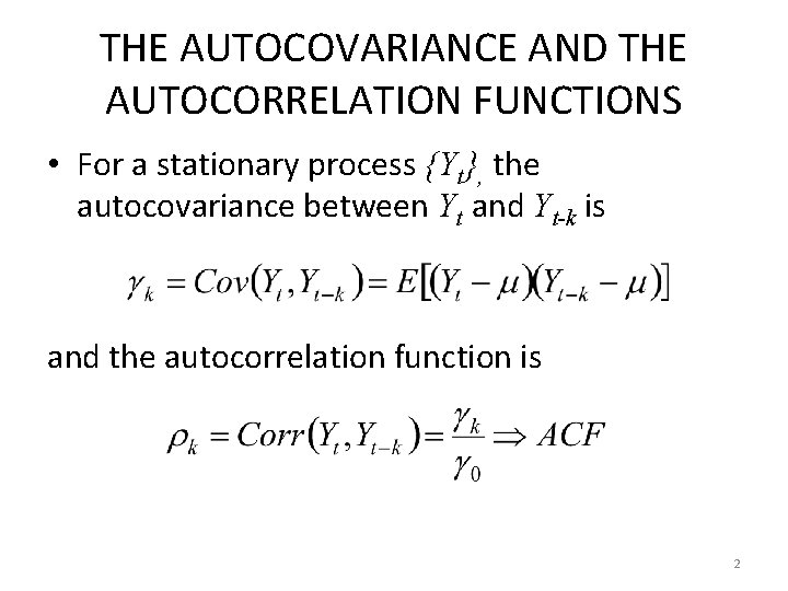
THE AUTOCOVARIANCE AND THE AUTOCORRELATION FUNCTIONS • For a stationary process {Yt}, the autocovariance between Yt and Yt-k is and the autocorrelation function is 2

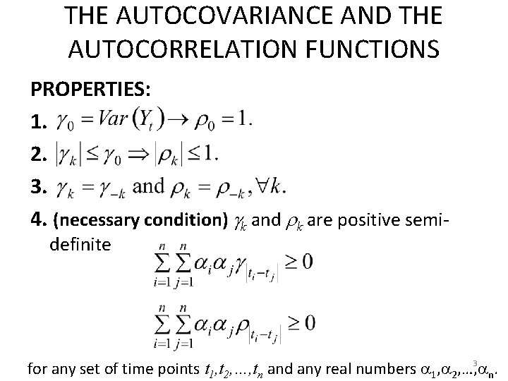
THE AUTOCOVARIANCE AND THE AUTOCORRELATION FUNCTIONS PROPERTIES: 1. 2. 3. 4. (necessary condition) k and k are positive semidefinite 3 for any set of time points t 1, t 2, …, tn and any real numbers 1, 2, …, n.

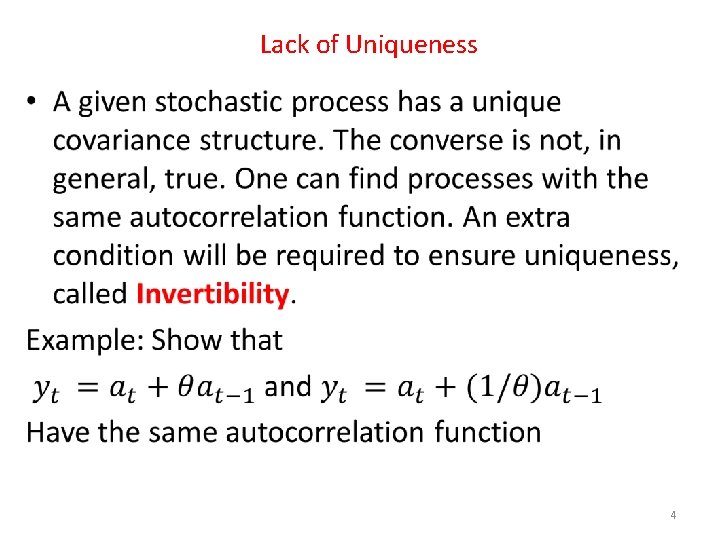
Lack of Uniqueness • 4

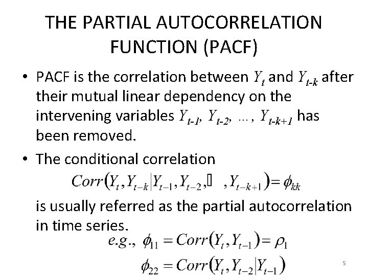
THE PARTIAL AUTOCORRELATION FUNCTION (PACF) • PACF is the correlation between Yt and Yt-k after their mutual linear dependency on the intervening variables Yt-1, Yt-2, …, Yt-k+1 has been removed. • The conditional correlation is usually referred as the partial autocorrelation in time series. 5

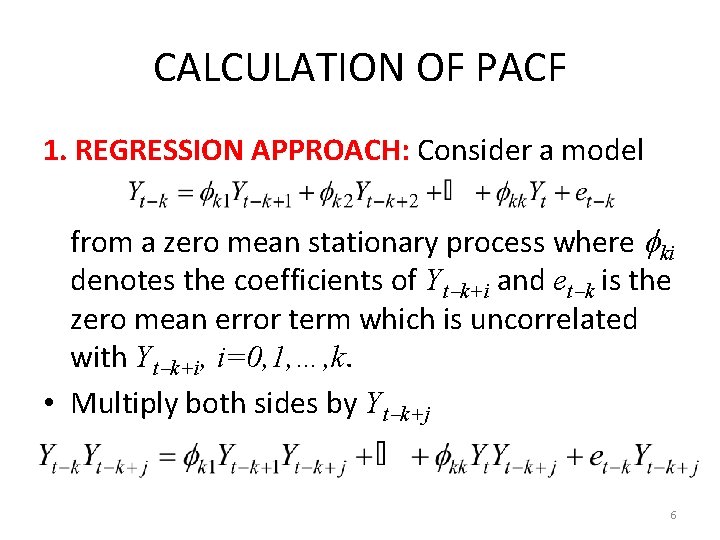
CALCULATION OF PACF 1. REGRESSION APPROACH: Consider a model from a zero mean stationary process where ki denotes the coefficients of Yt k+i and et k is the zero mean error term which is uncorrelated with Yt k+i, i=0, 1, …, k. • Multiply both sides by Yt k+j 6

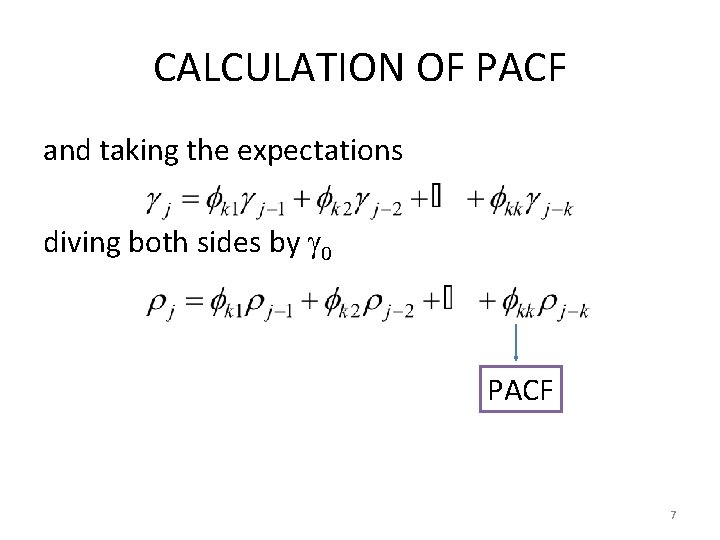
CALCULATION OF PACF and taking the expectations diving both sides by 0 PACF 7

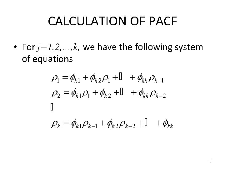
CALCULATION OF PACF • For j=1, 2, …, k, we have the following system of equations 8

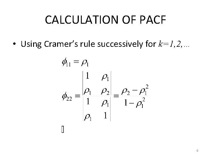
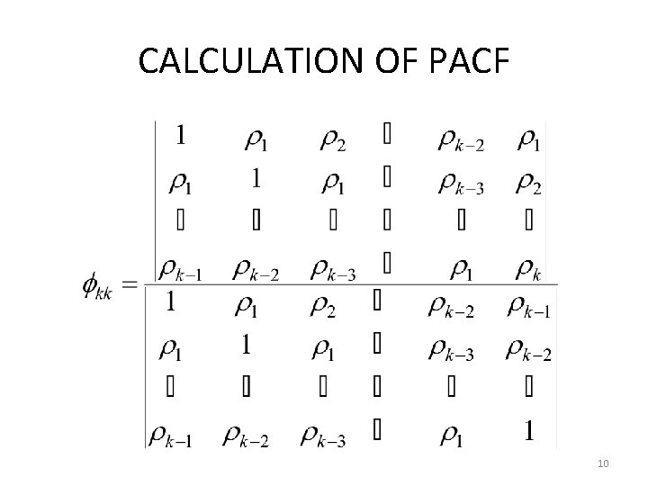
CALCULATION OF PACF • Using Cramer’s rule successively for k=1, 2, … 9

CALCULATION OF PACF 10

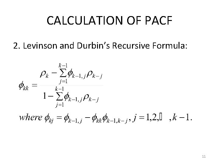
CALCULATION OF PACF 2. Levinson and Durbin’s Recursive Formula: 11

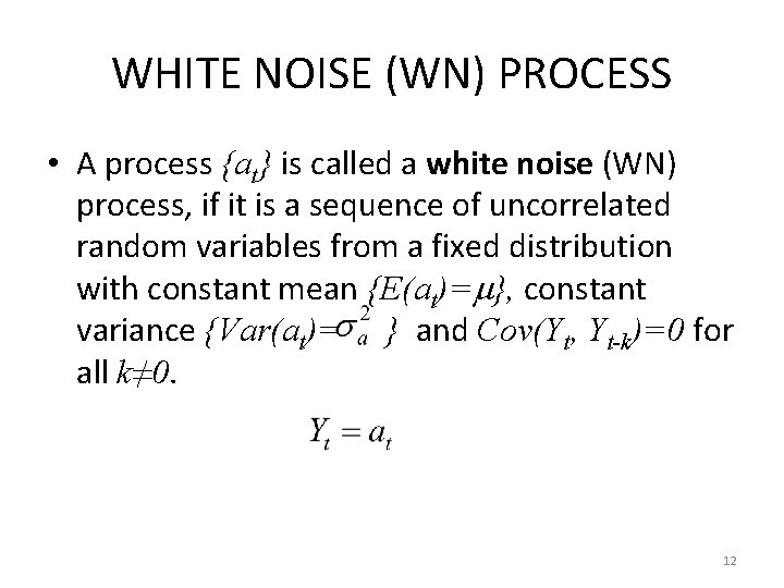
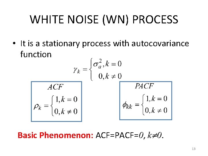
WHITE NOISE (WN) PROCESS • A process {at} is called a white noise (WN) process, if it is a sequence of uncorrelated random variables from a fixed distribution with constant mean {E(at)= }, constant variance {Var(at)= } and Cov(Yt, Yt-k)=0 for all k≠ 0. 12

WHITE NOISE (WN) PROCESS • It is a stationary process with autocovariance function Basic Phenomenon: ACF=PACF=0, k 0. 13

WHITE NOISE (WN) PROCESS • White noise (in spectral analysis): white light is produced in which all frequencies (i. e. , colors) are present in equal amount. • Memoryless process • Building block from which we can construct more complicated models • It plays the role of an orthogonal basis in the general vector and function analysis. 14

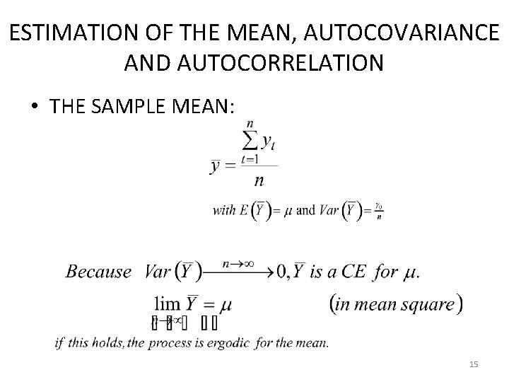
ESTIMATION OF THE MEAN, AUTOCOVARIANCE AND AUTOCORRELATION • THE SAMPLE MEAN: 15

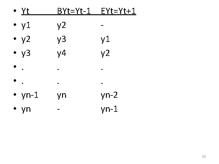
• • Yt y 1 y 2 y 3. . yn-1 yn BYt=Yt-1 y 2 y 3 y 4. . yn - EYt=Yt+1 y 2. . yn-2 yn-1 16

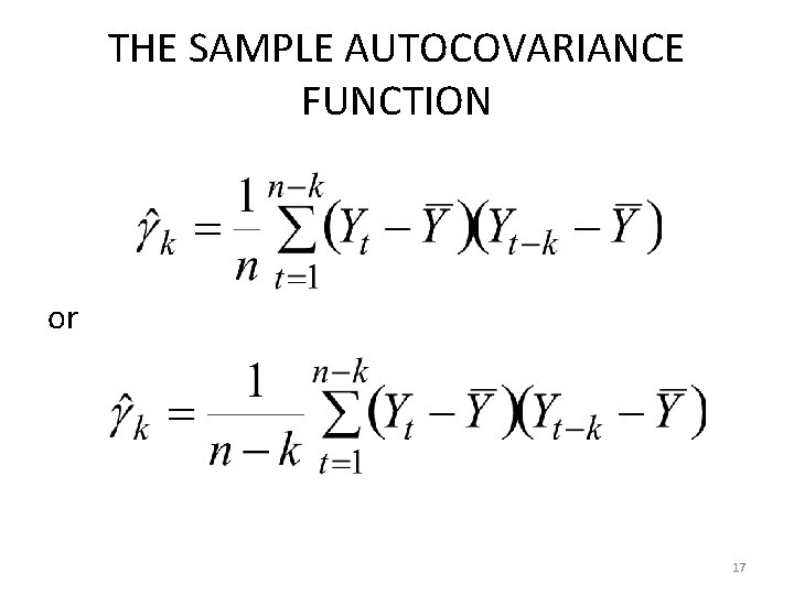
THE SAMPLE AUTOCOVARIANCE FUNCTION or 17

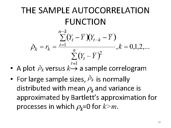
THE SAMPLE AUTOCORRELATION FUNCTION • A plot versus k a sample correlogram • For large sample sizes, is normally distributed with mean k and variance is approximated by Bartlett’s approximation for processes in which k=0 for k>m. 18

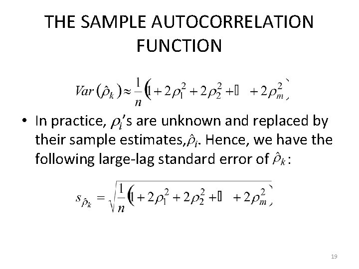
THE SAMPLE AUTOCORRELATION FUNCTION • In practice, i’s are unknown and replaced by their sample estimates, . Hence, we have the following large-lag standard error of : 19

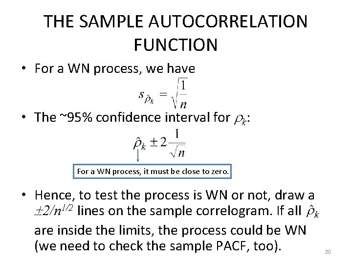
THE SAMPLE AUTOCORRELATION FUNCTION • For a WN process, we have • The ~95% confidence interval for k: For a WN process, it must be close to zero. • Hence, to test the process is WN or not, draw a 2/n 1/2 lines on the sample correlogram. If all are inside the limits, the process could be WN (we need to check the sample PACF, too). 20

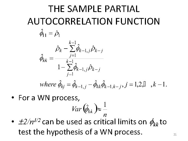
THE SAMPLE PARTIAL AUTOCORRELATION FUNCTION • For a WN process, • 2/n 1/2 can be used as critical limits on kk to test the hypothesis of a WN process. 21

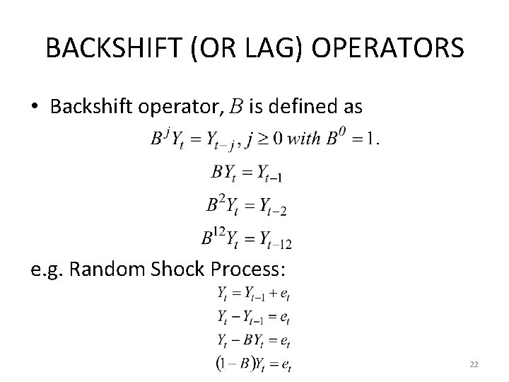
BACKSHIFT (OR LAG) OPERATORS • Backshift operator, B is defined as e. g. Random Shock Process: 22

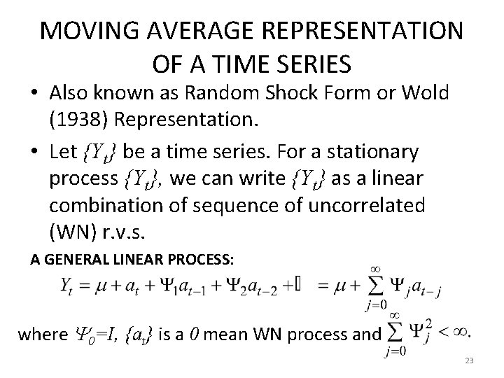
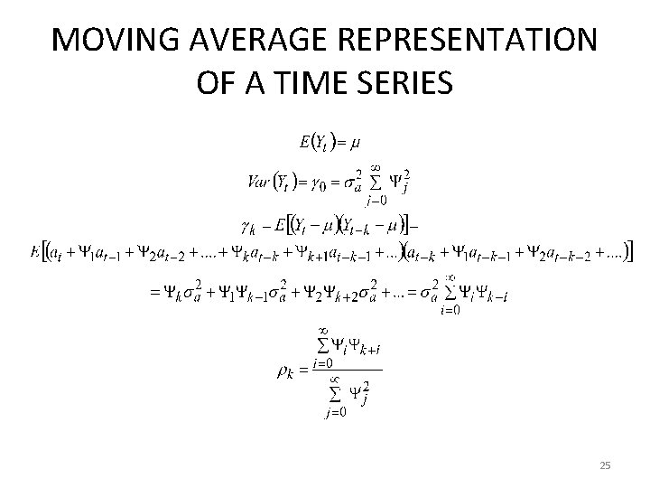
MOVING AVERAGE REPRESENTATION OF A TIME SERIES • Also known as Random Shock Form or Wold (1938) Representation. • Let {Yt} be a time series. For a stationary process {Yt}, we can write {Yt} as a linear combination of sequence of uncorrelated (WN) r. v. s. A GENERAL LINEAR PROCESS: where 0=I, {at} is a 0 mean WN process and 23

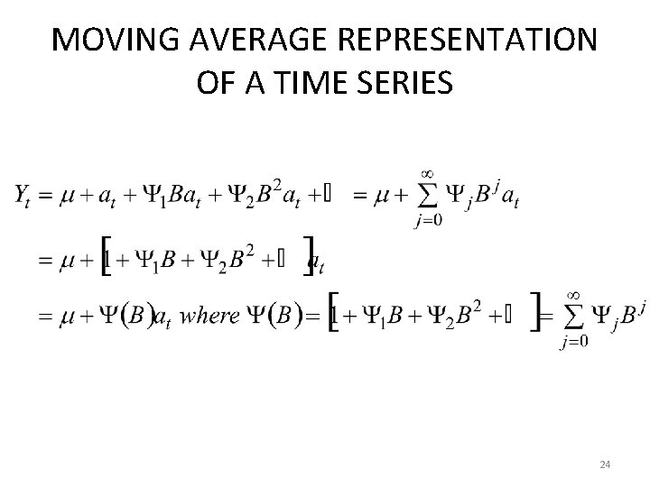
MOVING AVERAGE REPRESENTATION OF A TIME SERIES 24

MOVING AVERAGE REPRESENTATION OF A TIME SERIES 25

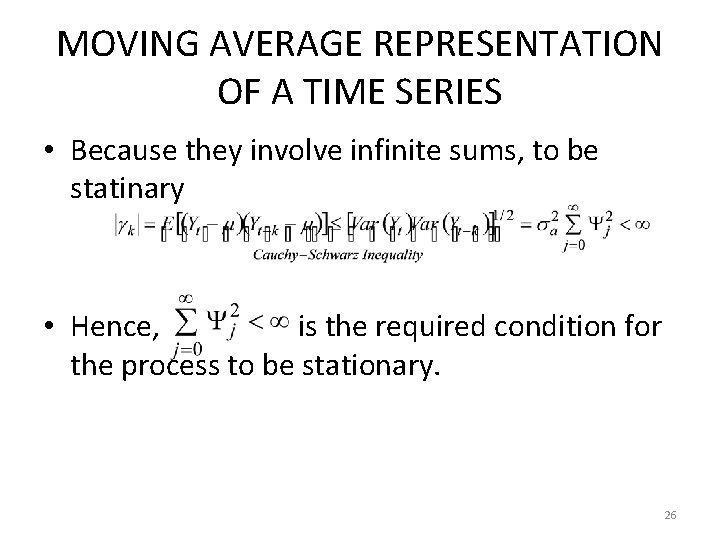
MOVING AVERAGE REPRESENTATION OF A TIME SERIES • Because they involve infinite sums, to be statinary • Hence, is the required condition for the process to be stationary. 26

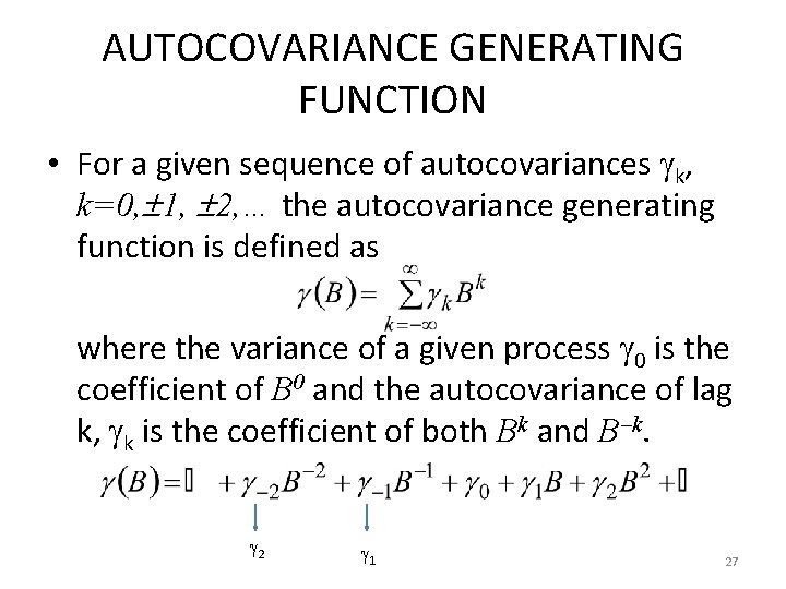
AUTOCOVARIANCE GENERATING FUNCTION • For a given sequence of autocovariances k, k=0, 1, 2, … the autocovariance generating function is defined as where the variance of a given process 0 is the coefficient of B 0 and the autocovariance of lag k, k is the coefficient of both Bk and B k. 2 1 27

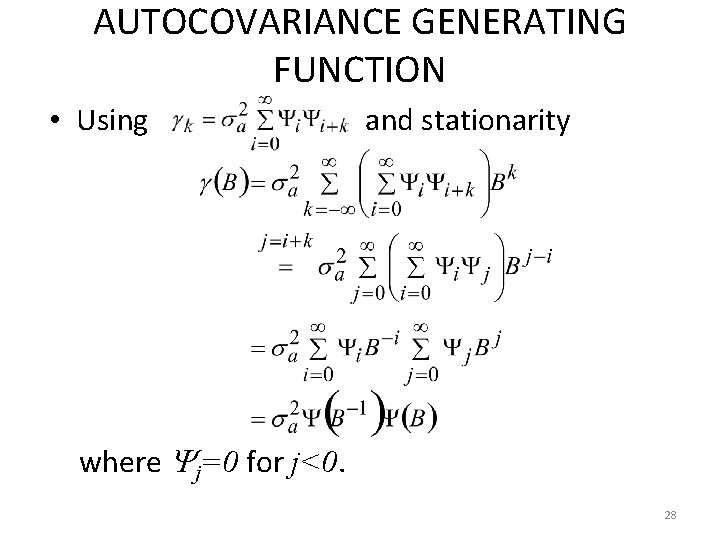
AUTOCOVARIANCE GENERATING FUNCTION • Using and stationarity where j=0 for j<0. 28

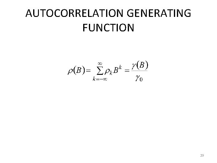
AUTOCORRELATION GENERATING FUNCTION 29

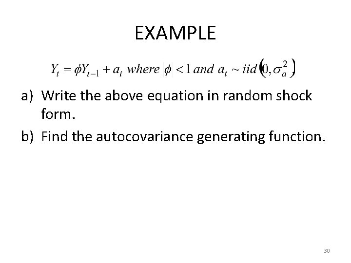
EXAMPLE a) Write the above equation in random shock form. b) Find the autocovariance generating function. 30

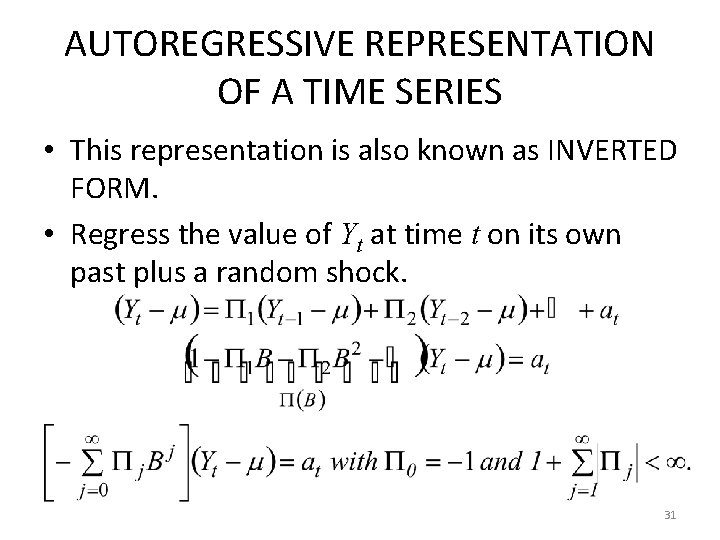
AUTOREGRESSIVE REPRESENTATION OF A TIME SERIES • This representation is also known as INVERTED FORM. • Regress the value of Yt at time t on its own past plus a random shock. 31

AUTOREGRESSIVE REPRESENTATION OF A TIME SERIES • It is an invertible process (it is important forecasting). Not every stationary process in invertible (Box and Jenkins, 1978). • Invertibility provides uniqueness of the autocorrelation function. • It means that different time series models can be re-expressed by each other. 32

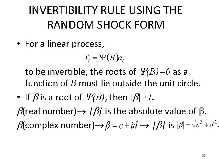
INVERTIBILITY RULE USING THE RANDOM SHOCK FORM • For a linear process, to be invertible, the roots of (B)=0 as a function of B must lie outside the unit circle. • If is a root of (B), then | |>1. (real number) | | is the absolute value of . (complex number) | | is 33

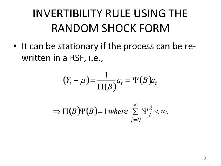
INVERTIBILITY RULE USING THE RANDOM SHOCK FORM • It can be stationary if the process can be rewritten in a RSF, i. e. , 34

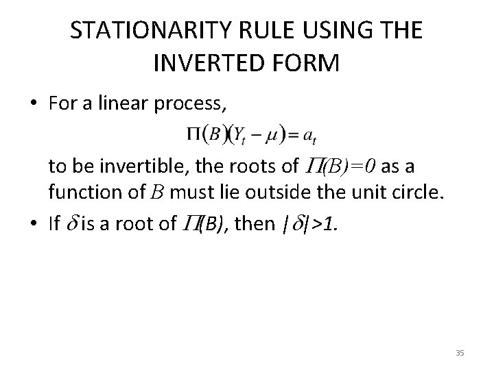
STATIONARITY RULE USING THE INVERTED FORM • For a linear process, to be invertible, the roots of (B)=0 as a function of B must lie outside the unit circle. • If is a root of (B), then | |>1. 35

RANDOM SHOCK FORM AND INVERTED FORM • AR and MA representations are not the model form. Because they contain infinite number of parameters that are impossible to estimate from a finite number of observations. 36

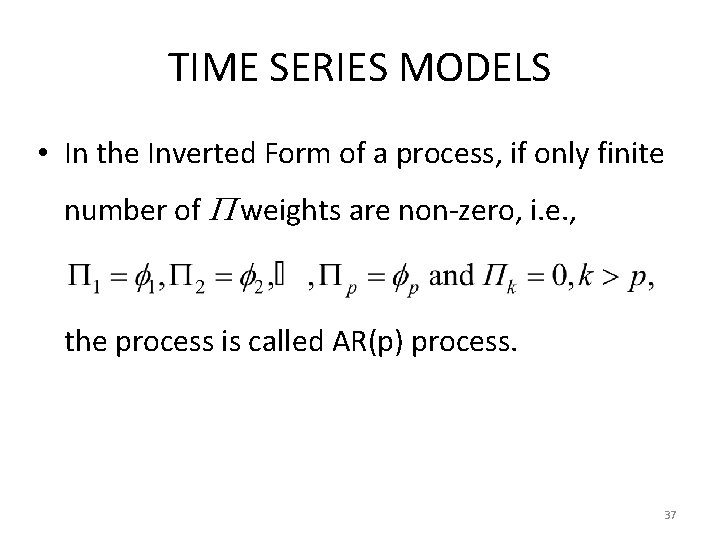
TIME SERIES MODELS • In the Inverted Form of a process, if only finite number of weights are non-zero, i. e. , the process is called AR(p) process. 37

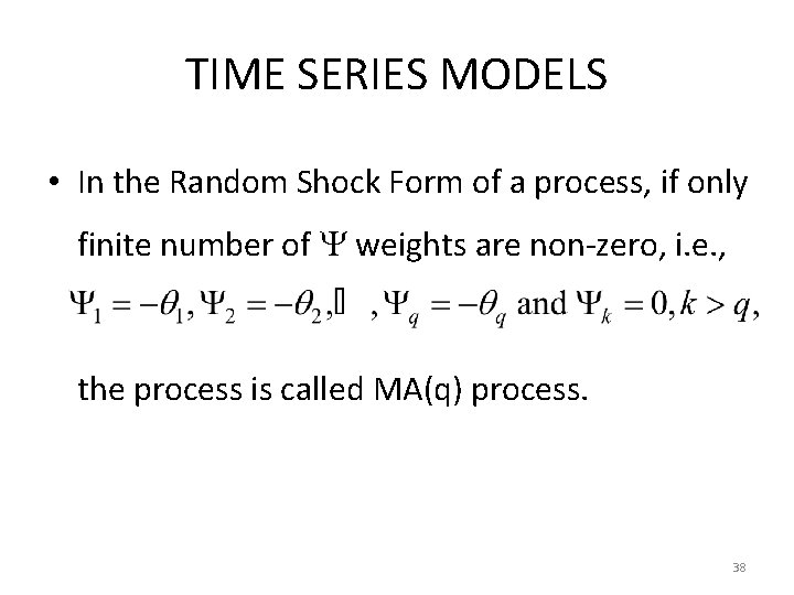
TIME SERIES MODELS • In the Random Shock Form of a process, if only finite number of weights are non-zero, i. e. , the process is called MA(q) process. 38

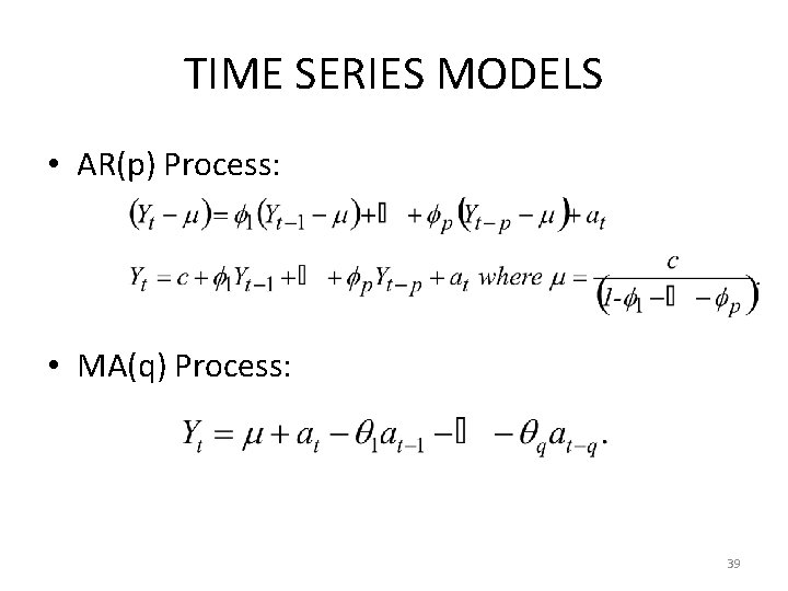
TIME SERIES MODELS • AR(p) Process: • MA(q) Process: 39

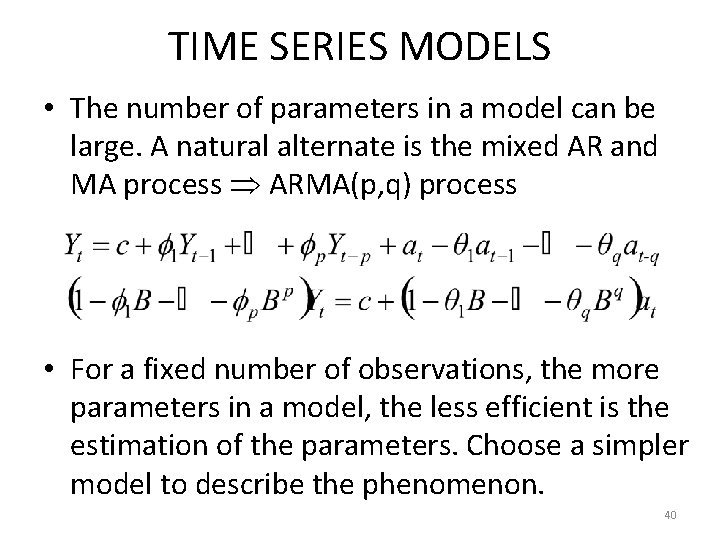
TIME SERIES MODELS • The number of parameters in a model can be large. A natural alternate is the mixed AR and MA process ARMA(p, q) process • For a fixed number of observations, the more parameters in a model, the less efficient is the estimation of the parameters. Choose a simpler model to describe the phenomenon. 40