STAT 497 LECTURE NOTES 8 TIME SERIES DECOMPOSITION

STAT 497 LECTURE NOTES 8 TIME SERIES DECOMPOSITION Classical decomposition, STL decomposition, detecting and correcting outliers in time series (https: //otexts. com/fpp 3/decomposition. html) 1

Time series decomposition • Time series data can exhibit a variety of patterns, and it is often helpful to split a time series into several components, each representing an underlying pattern category. • These patterns are trend, cycle and seasonal patterns. 2

Time series components • If we assume an additive decomposition, then we can write yt=St+Tt+Rt, where yt is the data, St is the seasonal component, Tt is the trend-cycle component, and Rt is the remainder component, all at period t. • Alternatively, a multiplicative decomposition would be written as yt=St×Tt×Rt. • The additive decomposition is the most appropriate if the magnitude of the seasonal fluctuations, or the variation around the trend-cycle, does not vary with the level of the time series. When the variation in the seasonal pattern, or the variation around the trend-cycle, appears to be proportional to the level of the time series, then a multiplicative decomposition is more appropriate. Multiplicative decompositions are common with economic time series. 3

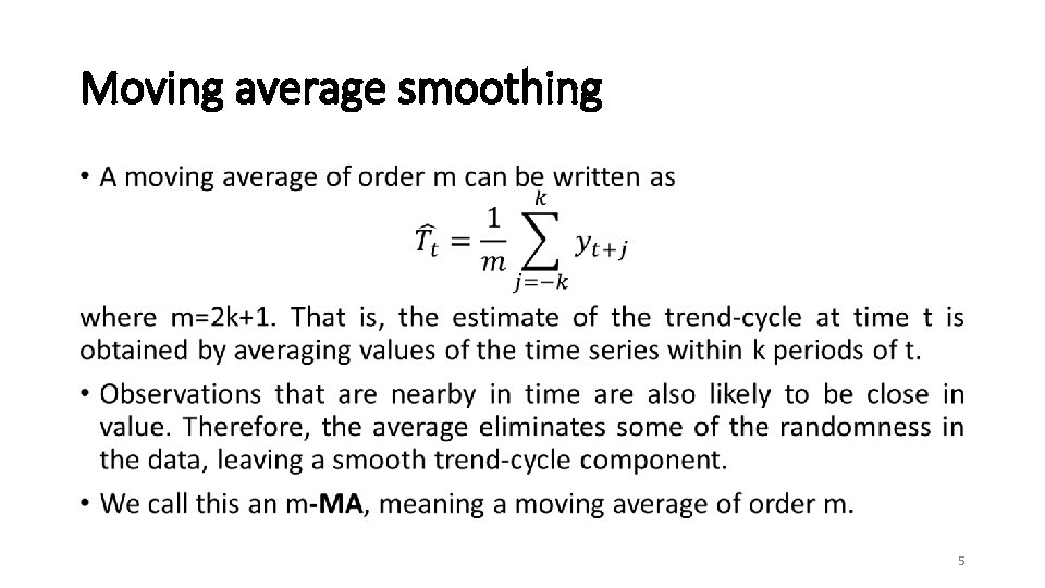
Moving averages • The classical method of time series decomposition originated in the 1920 s and was widely used until the 1950 s. It still forms the basis of many time series decomposition methods, so it is important to understand how it works. The first step in a classical decomposition is to use a moving average method to estimate the trend-cycle, so we begin by discussing moving averages. 4

Moving average smoothing • 5

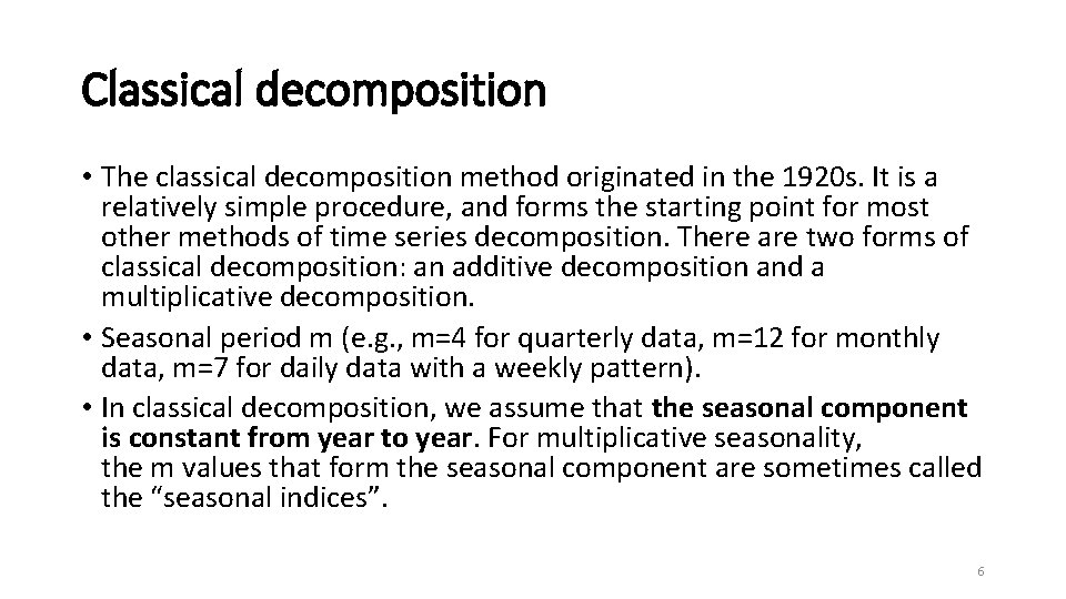
Classical decomposition • The classical decomposition method originated in the 1920 s. It is a relatively simple procedure, and forms the starting point for most other methods of time series decomposition. There are two forms of classical decomposition: an additive decomposition and a multiplicative decomposition. • Seasonal period m (e. g. , m=4 for quarterly data, m=12 for monthly data, m=7 for daily data with a weekly pattern). • In classical decomposition, we assume that the seasonal component is constant from year to year. For multiplicative seasonality, the m values that form the seasonal component are sometimes called the “seasonal indices”. 6

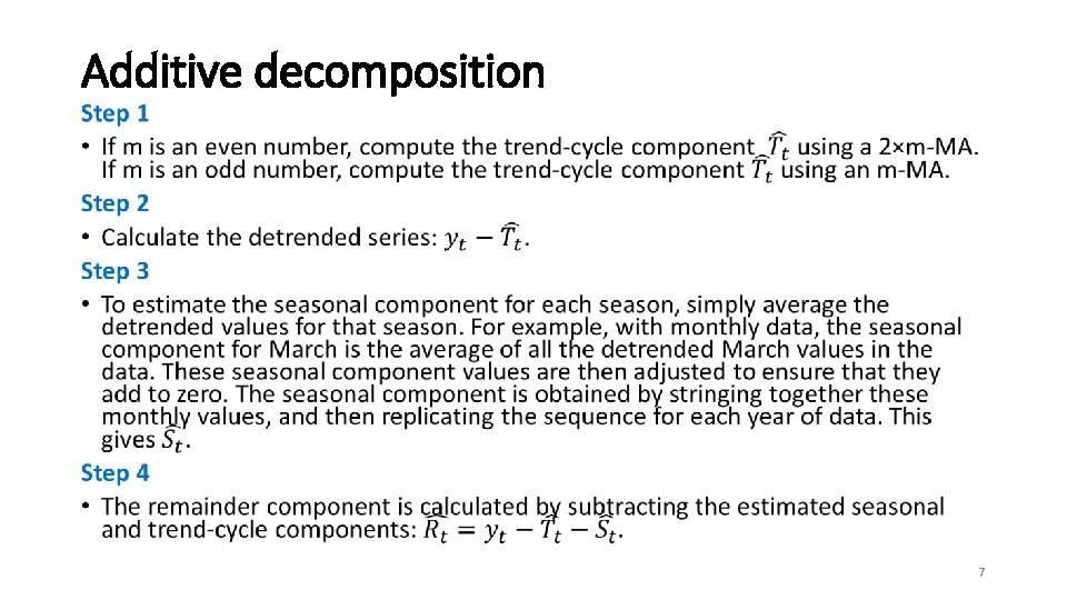
Additive decomposition • 7

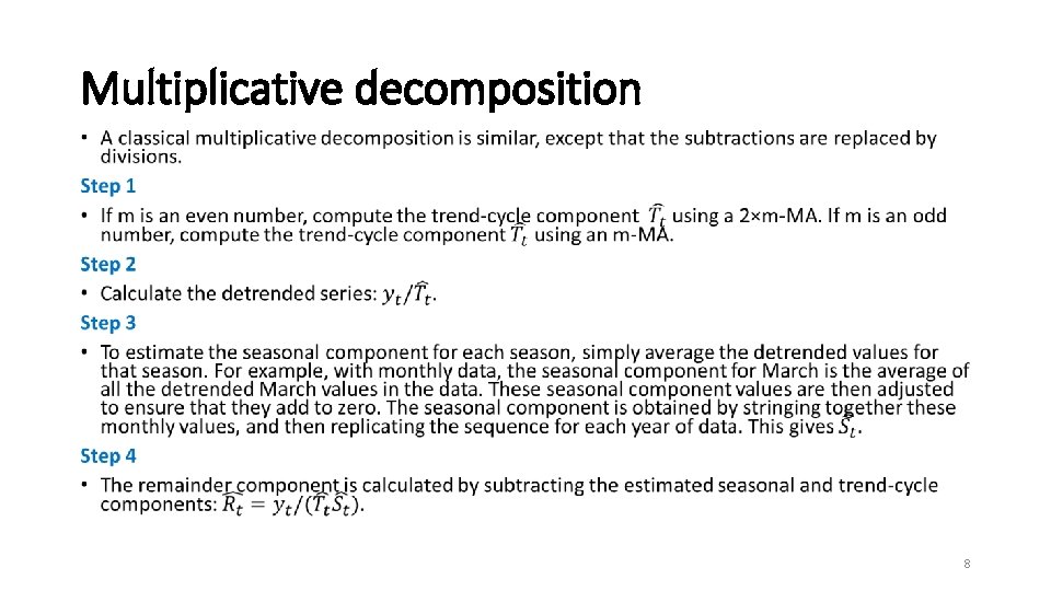
Multiplicative decomposition • 8

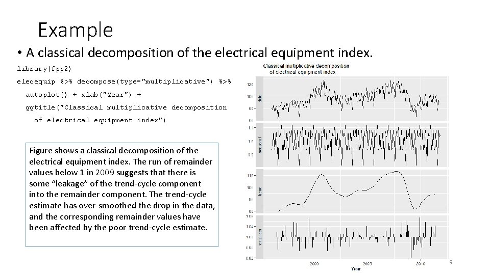
Example • A classical decomposition of the electrical equipment index. library(fpp 2) elecequip %>% decompose(type="multiplicative") %>% autoplot() + xlab("Year") + ggtitle("Classical multiplicative decomposition of electrical equipment index") Figure shows a classical decomposition of the electrical equipment index. The run of remainder values below 1 in 2009 suggests that there is some “leakage” of the trend-cycle component into the remainder component. The trend-cycle estimate has over-smoothed the drop in the data, and the corresponding remainder values have been affected by the poor trend-cycle estimate. 9

Comments on classical decomposition • While classical decomposition is still widely used, it is not recommended, as there are now several much better methods. • The estimate of the trend-cycle is unavailable for the first few and last few observations. For example, if m=12, there is no trend-cycle estimate for the first six or the last six observations. Consequently, there is also no estimate of the remainder component for the same time periods. • The trend-cycle estimate tends to over-smooth rapid rises and falls in the data. • Classical decomposition methods assume that the seasonal component repeats from year to year. For many series, this is a reasonable assumption, but for some longer series it is not. 10

STL decomposition • STL is a versatile and robust method for decomposing time series. STL is an acronym for “Seasonal and Trend decomposition using Loess”, while Loess is a method for estimating nonlinear relationships. The STL method was developed by Cleveland, Mc. Rae, Terpenning (1990). • STL has several advantages over the classical, SEATS and X 11 decomposition methods: • Unlike SEATS and X 11, STL will handle any type of seasonality, not only monthly and quarterly data. • The seasonal component is allowed to change over time, and the rate of change can be controlled by the user. • The smoothness of the trend-cycle can also be controlled by the user. • It can be robust to outliers. They will, however, affect the remainder component. 11

STL decomposition • On the other hand, STL has some disadvantages. In particular, it does not handle trading day or calendar variation automatically, and it only provides facilities for additive decompositions. • It is possible to obtain a multiplicative decomposition by first taking logs of the data, then back-transforming the components. Decompositions between additive and multiplicative can be obtained using a Box-Cox transformation of the data with 0<λ<1. A value of λ=0 corresponds to the multiplicative decomposition while λ=1 is equivalent to an additive decomposition. 12

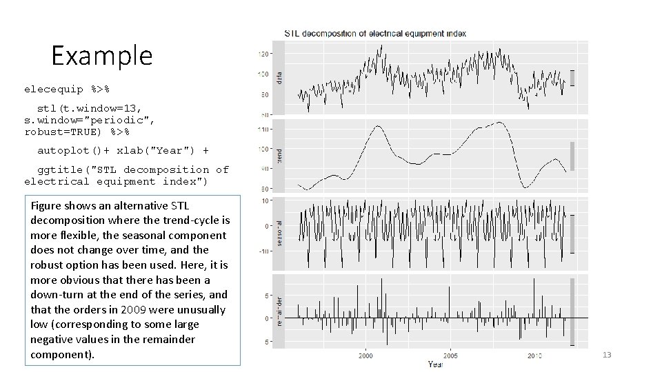
Example elecequip %>% stl(t. window=13, s. window="periodic", robust=TRUE) %>% autoplot()+ xlab("Year") + ggtitle("STL decomposition of electrical equipment index") Figure shows an alternative STL decomposition where the trend-cycle is more flexible, the seasonal component does not change over time, and the robust option has been used. Here, it is more obvious that there has been a down-turn at the end of the series, and that the orders in 2009 were unusually low (corresponding to some large negative values in the remainder component). 13

STL decomposition • The two main parameters to be chosen when using STL are the trend-cycle window (t. window) and the seasonal window (s. window). These control how rapidly the trend-cycle and seasonal components can change. Smaller values allow for more rapid changes. • Both t. window and s. window should be odd numbers; t. window is the number of consecutive observations to be used when estimating the trendcycle; s. window is the number of consecutive years to be used in estimating each value in the seasonal component. • The user must specify s. window as there is no default. Setting it to be infinite is equivalent to forcing the seasonal component to be periodic (i. e. , identical across years). Specifying t. window is optional, and a default value will be used if it is omitted. 14

STL decomposition • The mstl() function provides a convenient automated STL decomposition using s. window=13, and t. window also chosen automatically. This usually gives a good balance between overfitting the seasonality and allowing it to slowly change over time. But, as with any automated procedure, the default settings will need adjusting for some time series. 15

• We may easily extract the component time series: decomposed <- stl(time. series, s. window="periodic") seasonal trend remainder <- decomposed$time. series[, 1] <- decomposed$time. series[, 2] <- decomposed$time. series[, 3] This allows us to plot the seasonally-adjusted sales: plot(trend+remainder, main=“Seasonally Adjusted Series") 16

How stl() Works • When calling stl() with s. window="periodic", the seasonal component for January is simply the mean of all January values. Similarly, the seasonal component for February is simply the mean of all February values, etc. Otherwise, the seasonal component is calculated using loess smoothing. • Having calculated the seasonal component, the seasonally-adjusted data (the original data minus the seasonal component) is loesssmoothed to determine the trend. • The remainder/noise is then the original data minus the seasonal and trend components. 17

A LOES (or LOWES) Smoothing • Loess ("locally-weighted scatterplot smoothing") uses local regression to remove "jaggedness" from data. • A window of a specified width is placed over the data. The wider the window, the smoother the resulting loess curve. • A regression line (or curve) is fitted to the observations that fall within the window, the points closest to the center of the window being weighted to have the greatest effect on the calculation of the regression line. It uses nearest neighbor algorithm. • The weighting is reduced on those points within the window that are furthest from the regression line. The regression is re-run and weights are again re-calculated. This process is repeated several times. Weight can be define in a robust way by using medians. • We thereby obtain a point on the loess curve. This is the point on the regression line at the center of the window. • The loess curve is calculated by moving the window across the data. Each point on the resulting loess curve is the intersection of a regression line and a vertical line at the center of such a window. 18

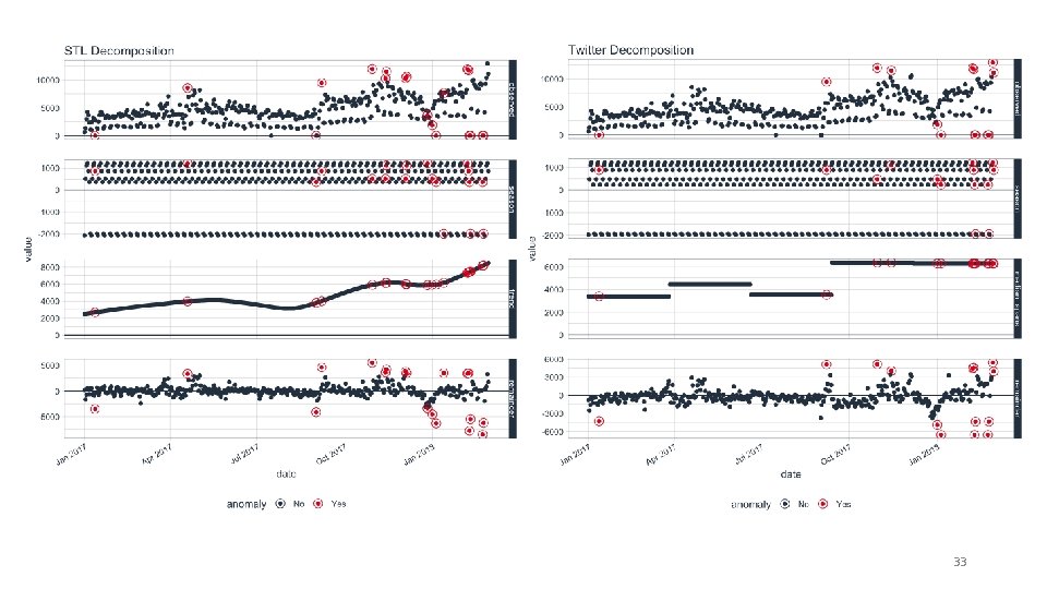
TWITTER METHOD • There is a second technique which you can use for seasonal decomposition in time series based on median: The Twitter method. • It is identical to STL for removing the seasonal component. The difference is in removing the trend is that it uses piece-wise median of the data (one or several median split at specified intervals) rather than fitting a smoother. This method works well where seasonality dominates the trend in time series. 19

STL vs TWITTER • STL works very well in circumstances where a long term trend is present. The Loess algorithm typically does a very good job at detecting the trend. However, it circumstances when the seasonal component is more dominant than the trend, Twitter tends to perform better. • The Twitter method works identically to STL for removing the seasonal component. The main difference is in removing the trend, which is performed by removing the median of the data rather than fitting a smoother. The median works well when a long-term trend is less dominant that the short-term seasonal component. This is because the smoother tends to overfit the anomalies. 20

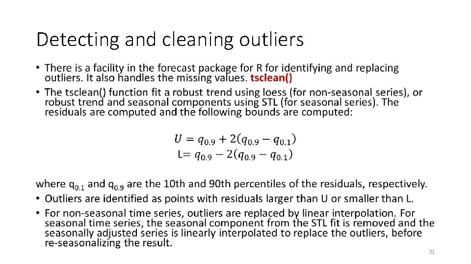
Detecting and cleaning outliers • 21

tsclean(): Identify and Replace Outliers and Missing Values in a Time Series • Uses supsmu (Scatter Plot Smoothing Using Super Smoother) for non-seasonal series and a robust STL decomposition for seasonal series. To estimate missing values and outlier replacements, linear interpolation is used on the (possibly seasonally adjusted) series. • While most smoothers require specification of a bandwidth, fraction of data, or level of smoothing, supersmoother is different in that it figures these things out for itself. Thus, it's an excellent choice for situations where smoothing needs to be done without any user intervention. Supersmoother works by performing lots of simple local regression smooths, and, at each x-value it uses those smooths to decide the best y-value to use. In R, supersmoother is made available through the supsmu function. • supsmu is a running lines smoother (Friedman's ‘super smoother’) which chooses between three spans for the lines. The running lines smoothers are symmetric, with k/2 data points each side of the predicted point, and values of k as 0. 5 * n , 0. 2 * n and 0. 05 * n , where n is the number of data points. 22

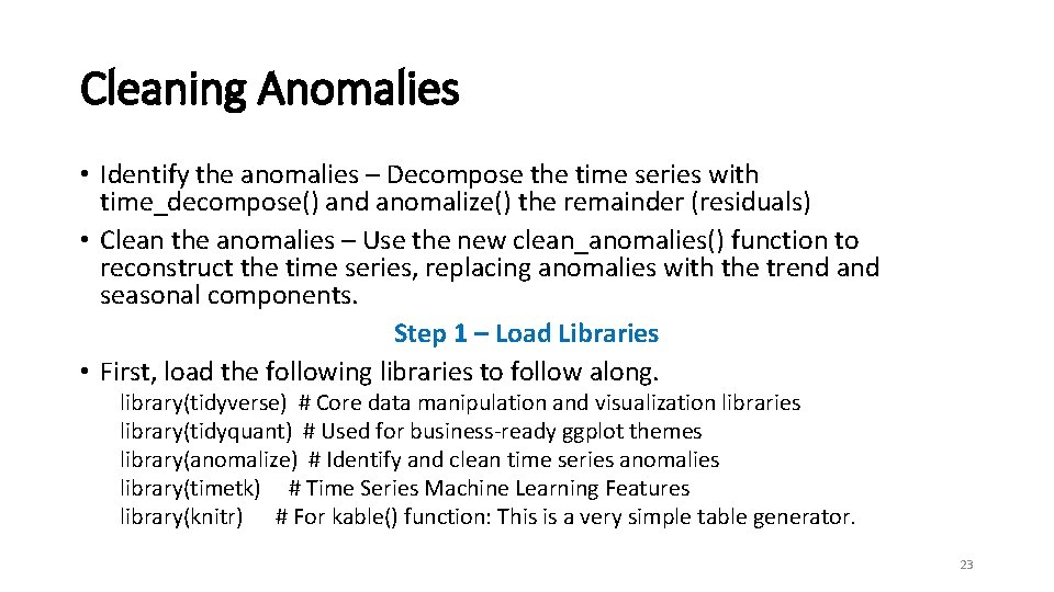
Cleaning Anomalies • Identify the anomalies – Decompose the time series with time_decompose() and anomalize() the remainder (residuals) • Clean the anomalies – Use the new clean_anomalies() function to reconstruct the time series, replacing anomalies with the trend and seasonal components. Step 1 – Load Libraries • First, load the following libraries to follow along. library(tidyverse) # Core data manipulation and visualization libraries library(tidyquant) # Used for business-ready ggplot themes library(anomalize) # Identify and clean time series anomalies library(timetk) # Time Series Machine Learning Features library(knitr) # For kable() function: This is a very simple table generator. 23

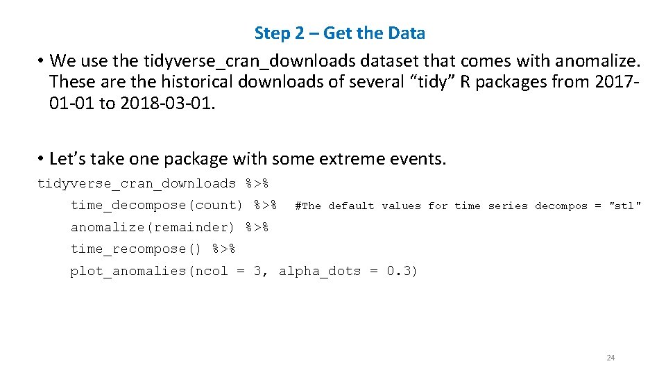
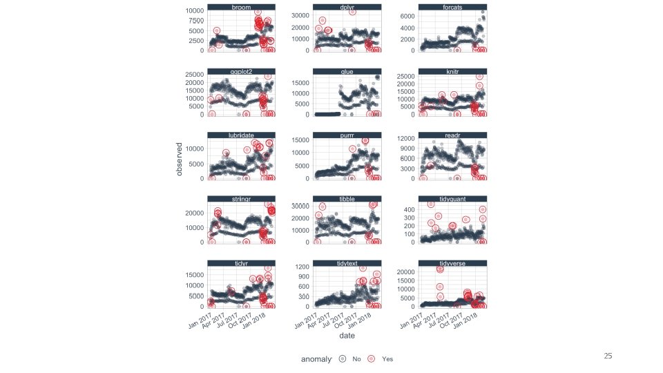
Step 2 – Get the Data • We use the tidyverse_cran_downloads dataset that comes with anomalize. These are the historical downloads of several “tidy” R packages from 201701 -01 to 2018 -03 -01. • Let’s take one package with some extreme events. tidyverse_cran_downloads %>% time_decompose(count) %>% #The default values for time series decompos = "stl" anomalize(remainder) %>% time_recompose() %>% plot_anomalies(ncol = 3, alpha_dots = 0. 3) 24

25

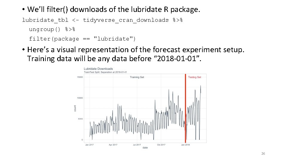
• We’ll filter() downloads of the lubridate R package. lubridate_tbl <- tidyverse_cran_downloads %>% ungroup() %>% filter(package == "lubridate") • Here’s a visual representation of the forecast experiment setup. Training data will be any data before “ 2018 -01 -01”. 26

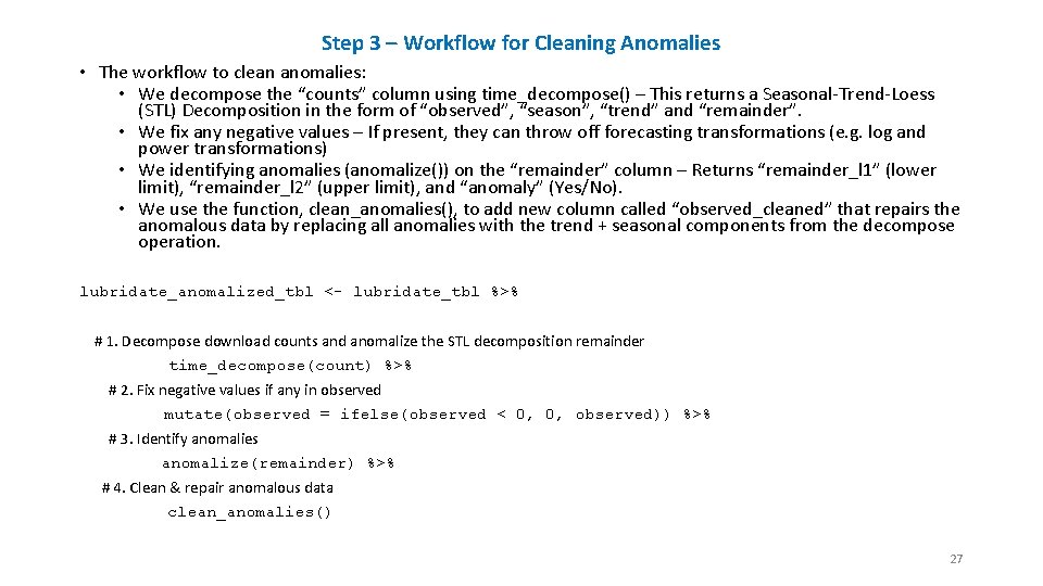
Step 3 – Workflow for Cleaning Anomalies • The workflow to clean anomalies: • We decompose the “counts” column using time_decompose() – This returns a Seasonal-Trend-Loess (STL) Decomposition in the form of “observed”, “season”, “trend” and “remainder”. • We fix any negative values – If present, they can throw off forecasting transformations (e. g. log and power transformations) • We identifying anomalies (anomalize()) on the “remainder” column – Returns “remainder_l 1” (lower limit), “remainder_l 2” (upper limit), and “anomaly” (Yes/No). • We use the function, clean_anomalies(), to add new column called “observed_cleaned” that repairs the anomalous data by replacing all anomalies with the trend + seasonal components from the decompose operation. lubridate_anomalized_tbl <- lubridate_tbl %>% # 1. Decompose download counts and anomalize the STL decomposition remainder time_decompose(count) %>% # 2. Fix negative values if any in observed mutate(observed = ifelse(observed < 0, 0, observed)) %>% # 3. Identify anomalies anomalize(remainder) %>% # 4. Clean & repair anomalous data clean_anomalies() 27

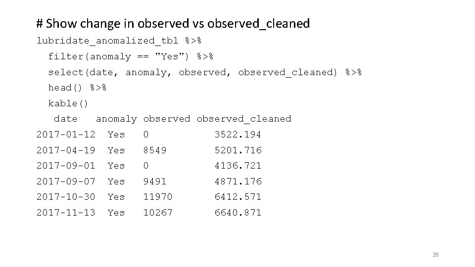
# Show change in observed vs observed_cleaned lubridate_anomalized_tbl %>% filter(anomaly == "Yes") %>% select(date, anomaly, observed_cleaned) %>% head() %>% kable() date anomaly observed_cleaned 2017 -01 -12 Yes 0 3522. 194 2017 -04 -19 Yes 8549 5201. 716 2017 -09 -01 Yes 0 4136. 721 2017 -09 -07 Yes 9491 4871. 176 2017 -10 -30 Yes 11970 6412. 571 2017 -11 -13 Yes 10267 6640. 871 28

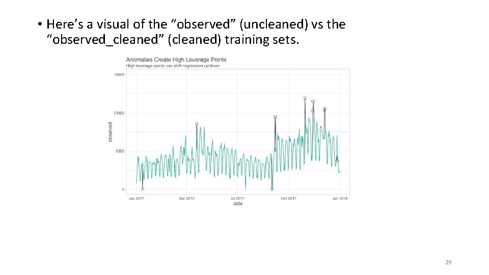
• Here’s a visual of the “observed” (uncleaned) vs the “observed_cleaned” (cleaned) training sets. 29

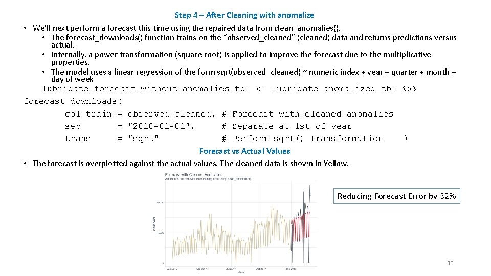
Step 4 – After Cleaning with anomalize • We’ll next perform a forecast this time using the repaired data from clean_anomalies(). • The forecast_downloads() function trains on the “observed_cleaned” (cleaned) data and returns predictions versus actual. • Internally, a power transformation (square-root) is applied to improve the forecast due to the multiplicative properties. • The model uses a linear regression of the form sqrt(observed_cleaned) ~ numeric index + year + quarter + month + day of week lubridate_forecast_without_anomalies_tbl <- lubridate_anomalized_tbl %>% forecast_downloads( col_train = observed_cleaned, # Forecast with cleaned anomalies sep = "2018 -01 -01", # Separate at 1 st of year trans = "sqrt" # Perform sqrt() transformation ) Forecast vs Actual Values • The forecast is overplotted against the actual values. The cleaned data is shown in Yellow. Reducing Forecast Error by 32% 30

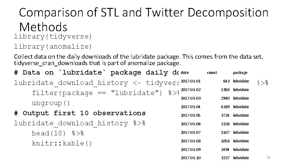
Comparison of STL and Twitter Decomposition Methods library(tidyverse) library(anomalize) Collect data on the daily downloads of the lubridate package. This comes from the data set, tidyverse_cran_downloads that is part of anomalize package. date count package # Data on `lubridate` package daily downloads 2017 -01 -01 643 lubridate_download_history <- tidyverse_cran_downloads %>% 2017 -01 -02 1350 lubridate filter(package == "lubridate") %>% 2017 -01 -03 2940 lubridate ungroup() 2017 -01 -04 4269 lubridate # Output first 10 observations 2017 -01 -05 3724 lubridate_download_history %>% 2017 -01 -06 2326 lubridate 2017 -01 -07 1107 lubridate head(10) %>% 2017 -01 -08 1058 lubridate knitr: : kable() 2017 -01 -09 2494 lubridate 2017 -01 -10 3237 lubridate 31

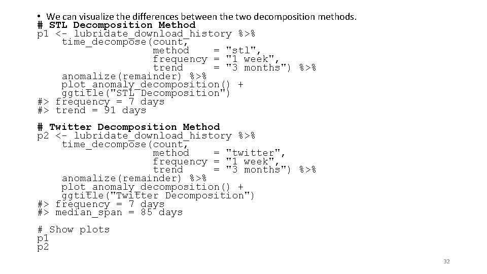
• We can visualize the differences between the two decomposition methods. # STL Decomposition Method p 1 <- lubridate_download_history %>% time_decompose(count, method = "stl", frequency = "1 week", trend = "3 months") %>% anomalize(remainder) %>% plot_anomaly_decomposition() + ggtitle("STL Decomposition") #> frequency = 7 days #> trend = 91 days # Twitter Decomposition Method p 2 <- lubridate_download_history %>% time_decompose(count, method = "twitter", frequency = "1 week", trend = "3 months") %>% anomalize(remainder) %>% plot_anomaly_decomposition() + ggtitle("Twitter Decomposition") #> frequency = 7 days #> median_span = 85 days # Show plots p 1 p 2 32

33

Detecting Anomalies in the Remainders • Once a time series analysis is completed and the remainder has the desired characteristics, the remainders can be analyzed. The challenge is that anomalies are high leverage points that distort the distribution. The anomalize package implements two methods that are resistant to the high leverage points: • IQR: Inner Quartile Range • GESD: Generalized Extreme Studentized Deviate Test • Both methods have pros and cons. 34

IQR • The IQR method is a similar method to that used in the forecast package for anomaly removal within the tsoutliers() function. It takes a distribution and uses the 25% and 75% inner quartile range to establish the distribution of the remainder. Limits are set by default to a factor of 3 X above and below the inner quartile range, and any remainders beyond the limits are considered anomalies. • The alpha parameter adjusts the 3 X factor. By default, alpha = 0. 05 for consistency with the GESD method. An alpha = 0. 025, results in a 6 X factor, expanding the limits and making it more difficult for data to be an anomaly. Conversely, an alpha = 0. 10 contracts the limits to a factor of 1. 5 X making it more easy for data to be an anomaly. • The IQR method does not depend on any loops and is therefore faster and more easily scaled than the GESD method. However, it may not be as accurate in detecting anomalies since the high leverage anomalies can skew the centerline (median) of the IQR 35

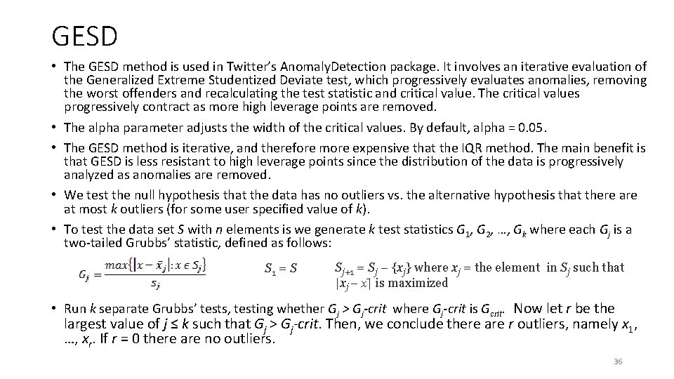
GESD • The GESD method is used in Twitter’s Anomaly. Detection package. It involves an iterative evaluation of the Generalized Extreme Studentized Deviate test, which progressively evaluates anomalies, removing the worst offenders and recalculating the test statistic and critical value. The critical values progressively contract as more high leverage points are removed. • The alpha parameter adjusts the width of the critical values. By default, alpha = 0. 05. • The GESD method is iterative, and therefore more expensive that the IQR method. The main benefit is that GESD is less resistant to high leverage points since the distribution of the data is progressively analyzed as anomalies are removed. • We test the null hypothesis that the data has no outliers vs. the alternative hypothesis that there at most k outliers (for some user specified value of k). • To test the data set S with n elements is we generate k test statistics G 1, G 2, …, Gk where each Gj is a two-tailed Grubbs’ statistic, defined as follows: S 1 = S Sj+1 = Sj − {xj} where xj = the element in Sj such that |xj − x | is maximized • Run k separate Grubbs’ tests, testing whether Gj > Gj-crit where Gj-crit is Gcrit. Now let r be the largest value of j ≤ k such that Gj > Gj-crit. Then, we conclude there are r outliers, namely x 1, …, xr. If r = 0 there are no outliers. 36

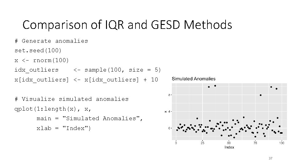
Comparison of IQR and GESD Methods # Generate anomalies set. seed(100) x <- rnorm(100) idx_outliers <- sample(100, size = 5) x[idx_outliers] <- x[idx_outliers] + 10 # Visualize simulated anomalies qplot(1: length(x), x, main = "Simulated Anomalies", xlab = "Index") 37

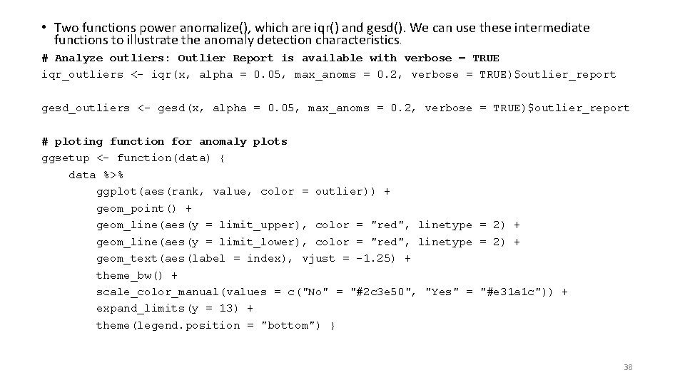
• Two functions power anomalize(), which are iqr() and gesd(). We can use these intermediate functions to illustrate the anomaly detection characteristics. # Analyze outliers: Outlier Report is available with verbose = TRUE iqr_outliers <- iqr(x, alpha = 0. 05, max_anoms = 0. 2, verbose = TRUE)$outlier_report gesd_outliers <- gesd(x, alpha = 0. 05, max_anoms = 0. 2, verbose = TRUE)$outlier_report # ploting function for anomaly plots ggsetup <- function(data) { data %>% ggplot(aes(rank, value, color = outlier)) + geom_point() + geom_line(aes(y = limit_upper), color = "red", linetype = 2) + geom_line(aes(y = limit_lower), color = "red", linetype = 2) + geom_text(aes(label = index), vjust = -1. 25) + theme_bw() + scale_color_manual(values = c("No" = "#2 c 3 e 50", "Yes" = "#e 31 a 1 c")) + expand_limits(y = 13) + theme(legend. position = "bottom") } 38

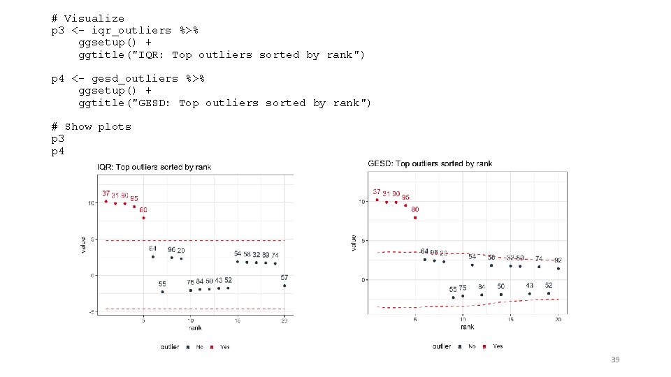
# Visualize p 3 <- iqr_outliers %>% ggsetup() + ggtitle("IQR: Top outliers sorted by rank") p 4 <- gesd_outliers %>% ggsetup() + ggtitle("GESD: Top outliers sorted by rank") # Show plots p 3 p 4 39

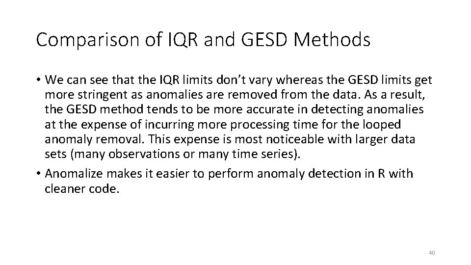
Comparison of IQR and GESD Methods • We can see that the IQR limits don’t vary whereas the GESD limits get more stringent as anomalies are removed from the data. As a result, the GESD method tends to be more accurate in detecting anomalies at the expense of incurring more processing time for the looped anomaly removal. This expense is most noticeable with larger data sets (many observations or many time series). • Anomalize makes it easier to perform anomaly detection in R with cleaner code. 40

Detecting multiple anomalies in seasonal time series (https: //www. r-bloggers. com/anomalydetection-in-r-2/) • Anomalies are essentially the outliers in our data. If something happens regularly, it is not an anomaly but a trend. Things which happen once or twice and are deviant from the usual behavior, whether continuously or with lags are all anomalies. • The Anomaly. Detection package is capable of identifying outliers in the presence of seasonality and trend in the data. The package uses an algorithm known as Seasonal Hybrid Extreme Studentized Deviate (ESD) algorithm which finds outliers globally as well as locally in time series or a vector of data. 41

Detecting multiple anomalies in seasonal time series install. packages("devtools") devtools: : install_github("twitter/Anomaly. Detection") library(Anomaly. Detection) Anomaly. Detection. Vec(x , period = 12, direction = 'both') Arguments x: vector of values period: period of repeating pattern direction: find anomalies that are small ('neg'), large ('pos'), or both ('both') 42

#Install the devtools package then github packages install. packages("devtools") install. packages("Rcpp") library(devtools) install_github("petermeissner/wikipediatrend") install_github("twitter/Anomaly. Detection") library(Rcpp) library(wikipediatrend) library(Anomaly. Detection) 43

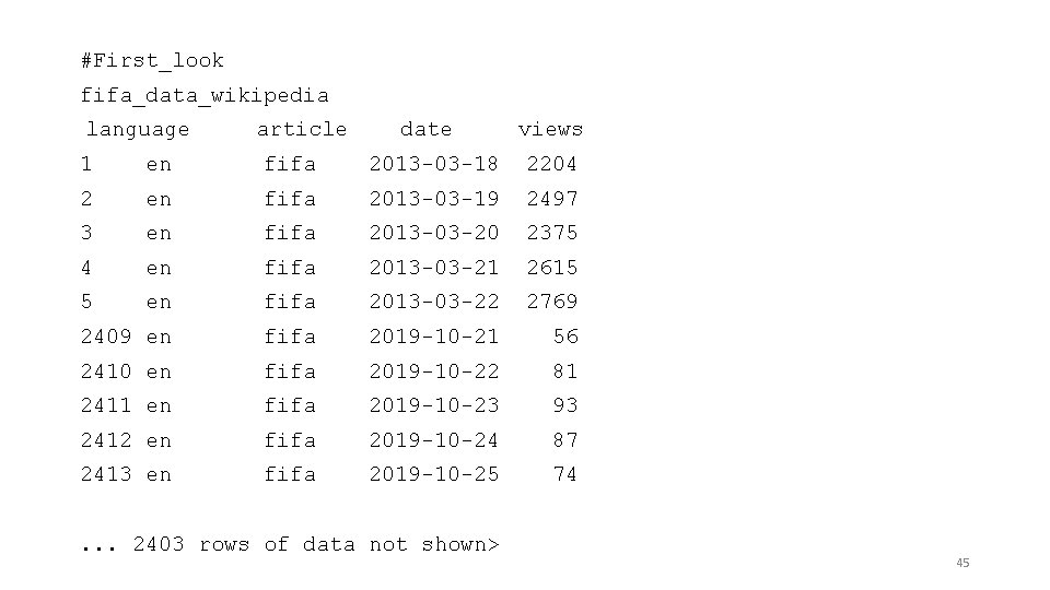
The first step is data preparation. We will use the page views on wikipedia page marked on fifa data starting from date 18 th March 2013. (link: https: //en. wikipedia. org/wiki/FIFA). The wp_trend function gives us the access statistics for the page with the ability to filter data from within the function. We will use this data to model day wise page views and understand anomalies in the pattern of those view numbers #Download wikipedia webpage "fifa" fifa_data_wikipedia = wp_trend("fifa", from="2013 -03 -18", lang = "en") This gives us a dataset of about 2413 observations and 5 columns. 44

#First_look fifa_data_wikipedia language article date views 1 en fifa 2013 -03 -18 2204 2 en fifa 2013 -03 -19 2497 3 en fifa 2013 -03 -20 2375 4 en fifa 2013 -03 -21 2615 5 en fifa 2013 -03 -22 2769 2409 en fifa 2019 -10 -21 56 2410 en fifa 2019 -10 -22 81 2411 en fifa 2019 -10 -23 93 2412 en fifa 2019 -10 -24 87 2413 en fifa 2019 -10 -25 74 . . . 2403 rows of data not shown> 45

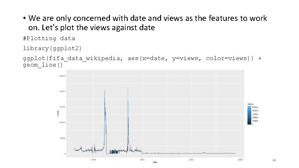
• We are only concerned with date and views as the features to work on. Let’s plot the views against date #Plotting data library(ggplot 2) ggplot(fifa_data_wikipedia, aes(x=date, y=views, color=views)) + geom_line() 46

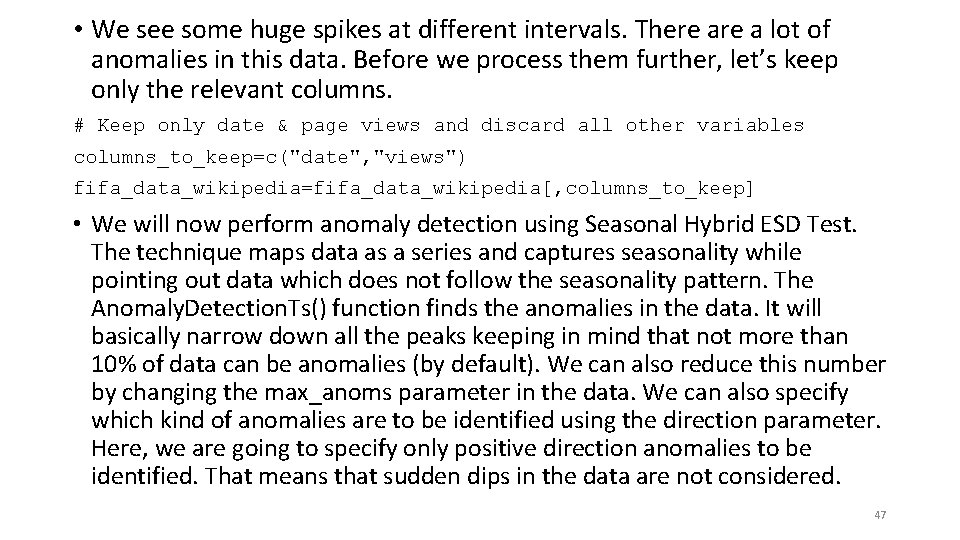
• We see some huge spikes at different intervals. There a lot of anomalies in this data. Before we process them further, let’s keep only the relevant columns. # Keep only date & page views and discard all other variables columns_to_keep=c("date", "views") fifa_data_wikipedia=fifa_data_wikipedia[, columns_to_keep] • We will now perform anomaly detection using Seasonal Hybrid ESD Test. The technique maps data as a series and captures seasonality while pointing out data which does not follow the seasonality pattern. The Anomaly. Detection. Ts() function finds the anomalies in the data. It will basically narrow down all the peaks keeping in mind that not more than 10% of data can be anomalies (by default). We can also reduce this number by changing the max_anoms parameter in the data. We can also specify which kind of anomalies are to be identified using the direction parameter. Here, we are going to specify only positive direction anomalies to be identified. That means that sudden dips in the data are not considered. 47

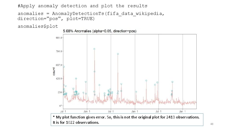
#Apply anomaly detection and plot the results anomalies = Anomaly. Detection. Ts(fifa_data_wikipedia, direction="pos", plot=TRUE) anomalies$plot * My plot function gives error. So, this is not the original plot for 2413 observations. It is for 1022 observations. 48

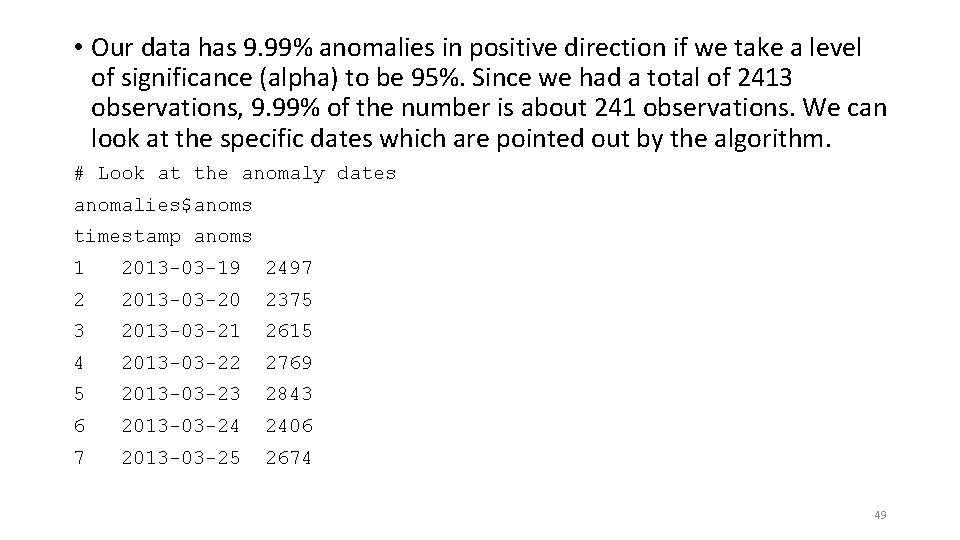
• Our data has 9. 99% anomalies in positive direction if we take a level of significance (alpha) to be 95%. Since we had a total of 2413 observations, 9. 99% of the number is about 241 observations. We can look at the specific dates which are pointed out by the algorithm. # Look at the anomaly dates anomalies$anoms timestamp anoms 1 2013 -03 -19 2497 2 2013 -03 -20 2375 3 2013 -03 -21 2615 4 2013 -03 -22 2769 5 2013 -03 -23 2843 6 2013 -03 -24 2406 7 2013 -03 -25 2674 49

• We have the exact dates and the anomaly values for each date. In a typical anomaly detection process, each of these dates are looked case by case and the reason for anomalies is identified. For instance, the page views can be higher on these dates if there had been fifa matches or page updates on these particular days. Another reason could be big news about fifa players. However, if page views on any of the dates does not correspond to any special event, then those days are true anomalies and should be flagged. In other situations such as credit card transactions, such anomalies can indicate fraud and quick action must be taken on identification. 50