STAT 497 LECTURE NOTE 15 REGRESSION WITH TIME

STAT 497 LECTURE NOTE 15 REGRESSION WITH TIME SERIES VARIABLES From Lecture Notes of Gary Koop, and Heino Bohn Nielsen and https: //www. udel. edu/htr/Statistics/Notes 816/class 20. PDF, http: //www. eco. uc 3 m. es/~jgonzalo/teaching/Tecnicas. Econometricas/ Wooldridge. Ch 10 -12. pdf 1

INTRODUCTION • Goal of regression modelling is complicated when the researcher uses time series data since an explanatory variable may influence a dependent variable with a time lag. This often necessitates the inclusion of lags of the explanatory variable in the regression. • If “time” is the unit of analysis, we can still regress some dependent variable, Y, on one or more independent variables. 2

Why use time series data? • To develop forecasting models • What will the rate of inflation be next year? • To estimate dynamic causal effects • If the Fed increases the Federal Funds rate now, what will be the effect on the rates of inflation and unemployment in 3 months? in 12 months? • What is the effect over time on cigarette consumption of a hike in the cigarette tax? • Or, because that is your only option … • Rates of inflation and unemployment in the US can be observed only over time 3

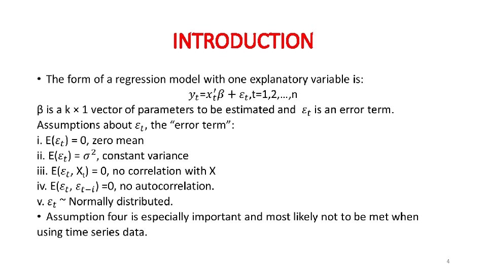
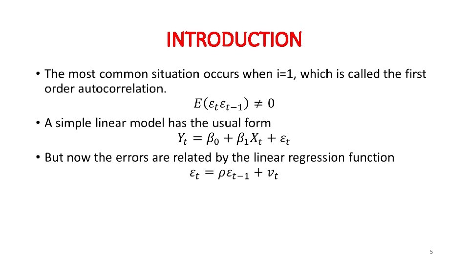
INTRODUCTION • 4

INTRODUCTION • 5

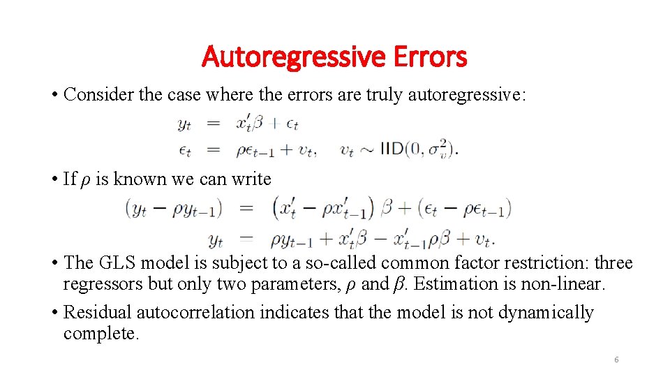
Autoregressive Errors • Consider the case where the errors are truly autoregressive: • If ρ is known we can write • The GLS model is subject to a so-called common factor restriction: three regressors but only two parameters, ρ and β. Estimation is non-linear. • Residual autocorrelation indicates that the model is not dynamically complete. 6

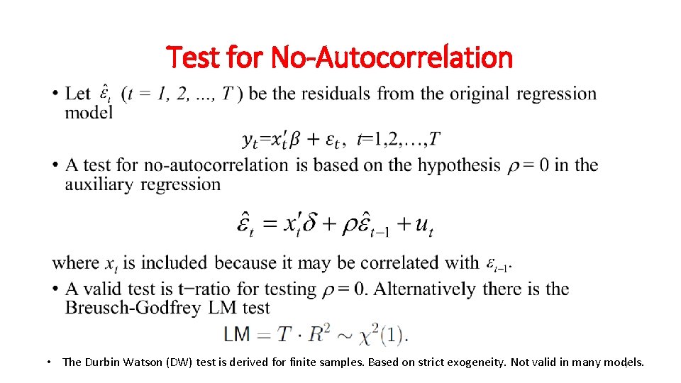
Test for No-Autocorrelation • • The Durbin Watson (DW) test is derived for finite samples. Based on strict exogeneity. Not valid in many models. 7

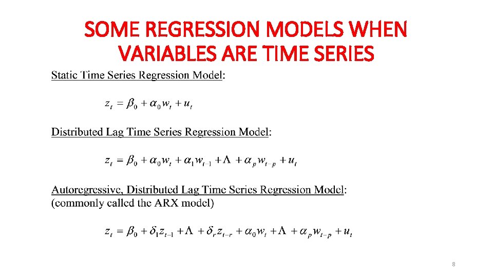
SOME REGRESSION MODELS WHEN VARIABLES ARE TIME SERIES 8

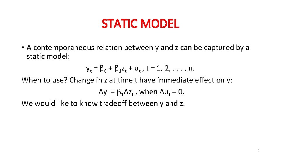
STATIC MODEL • A contemporaneous relation between y and z can be captured by a static model: yt = β 0 + β 1 zt + ut , t = 1, 2, . . . , n. When to use? Change in z at time t have immediate effect on y: ∆yt = β 1∆zt , when ∆ut = 0. We would like to know tradeoff between y and z. 9

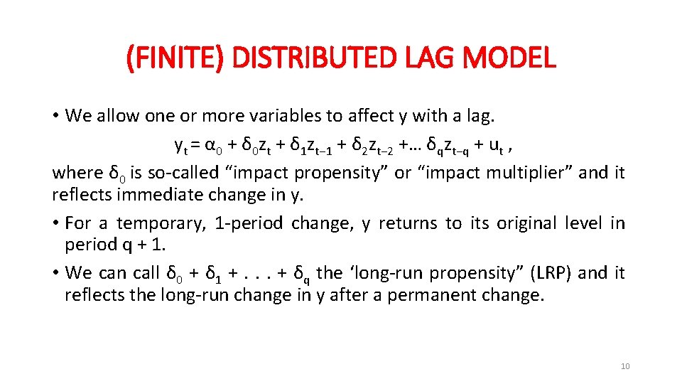
(FINITE) DISTRIBUTED LAG MODEL • We allow one or more variables to affect y with a lag. yt = α 0 + δ 0 zt + δ 1 zt− 1 + δ 2 zt− 2 +… δqzt−q + ut , where δ 0 is so-called “impact propensity” or “impact multiplier” and it reflects immediate change in y. • For a temporary, 1 -period change, y returns to its original level in period q + 1. • We can call δ 0 + δ 1 +. . . + δq the ‘long-run propensity” (LRP) and it reflects the long-run change in y after a permanent change. 10

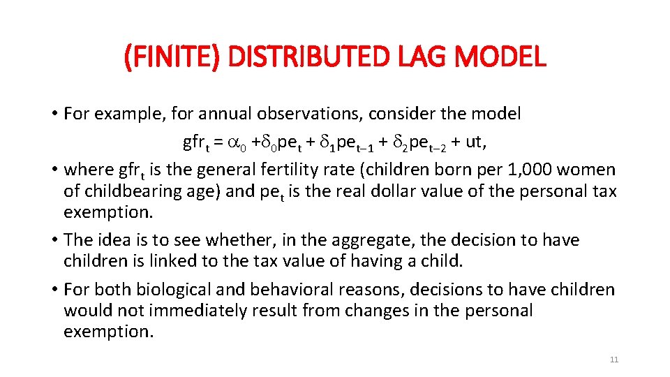
(FINITE) DISTRIBUTED LAG MODEL • For example, for annual observations, consider the model gfrt = 0 + 0 pet + 1 pet 1 + 2 pet 2 + ut, • where gfrt is the general fertility rate (children born per 1, 000 women of childbearing age) and pet is the real dollar value of the personal tax exemption. • The idea is to see whether, in the aggregate, the decision to have children is linked to the tax value of having a child. • For both biological and behavioral reasons, decisions to have children would not immediately result from changes in the personal exemption. 11

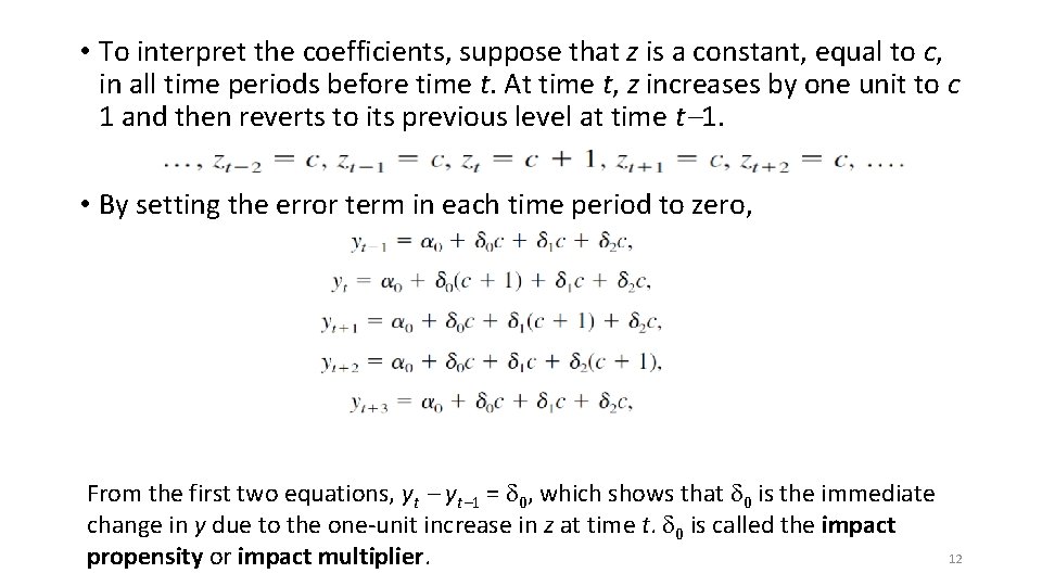
• To interpret the coefficients, suppose that z is a constant, equal to c, in all time periods before time t. At time t, z increases by one unit to c 1 and then reverts to its previous level at time t 1. • By setting the error term in each time period to zero, From the first two equations, yt 1 = 0, which shows that 0 is the immediate change in y due to the one-unit increase in z at time t. 0 is called the impact propensity or impact multiplier. 12

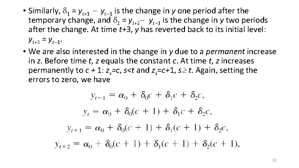
• Similarly, 1 = yt+1 yt 1 is the change in y one period after the temporary change, and 2 = yt+2 yt 1 is the change in y two periods after the change. At time t+3, y has reverted back to its initial level: yt+3 = yt 1. • We are also interested in the change in y due to a permanent increase in z. Before time t, z equals the constant c. At time t, z increases permanently to c + 1: zs=c, s<t and zs=c+1, s t. Again, setting the errors to zero, we have 13

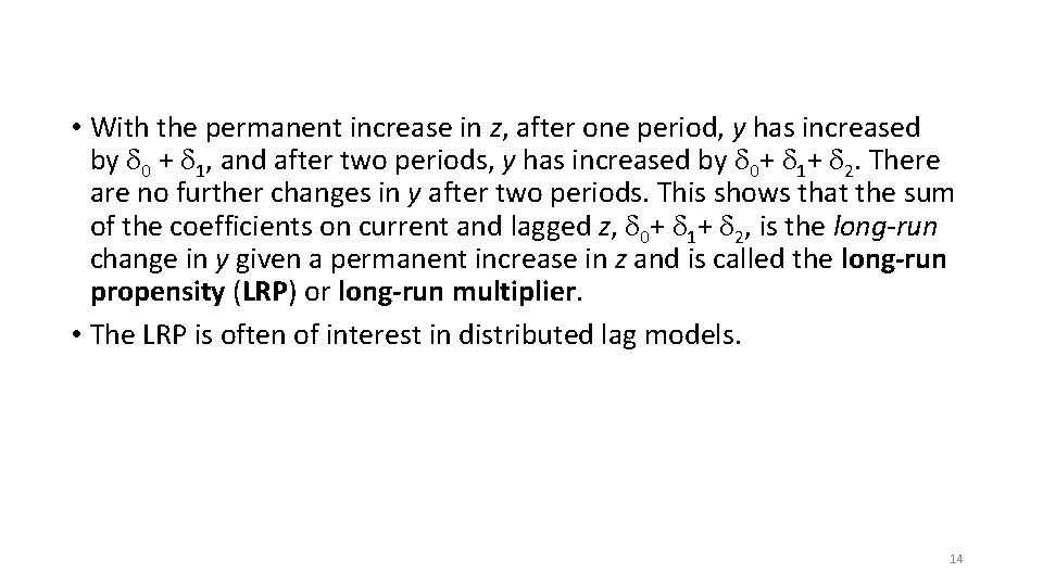
• With the permanent increase in z, after one period, y has increased by 0 + 1, and after two periods, y has increased by 0+ 1+ 2. There are no further changes in y after two periods. This shows that the sum of the coefficients on current and lagged z, 0+ 1+ 2, is the long-run change in y given a permanent increase in z and is called the long-run propensity (LRP) or long-run multiplier. • The LRP is often of interest in distributed lag models. 14

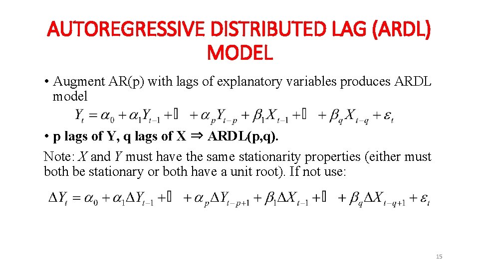
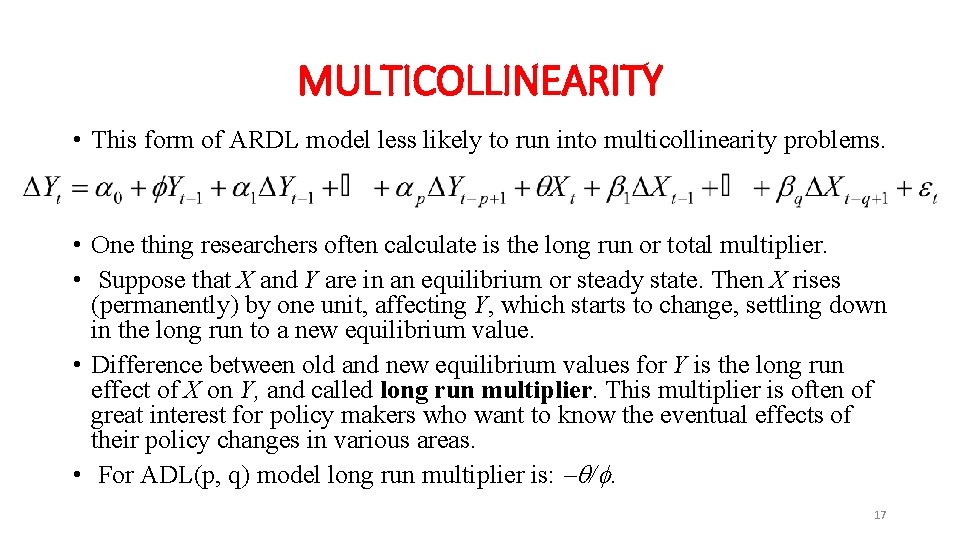
AUTOREGRESSIVE DISTRIBUTED LAG (ARDL) MODEL • Augment AR(p) with lags of explanatory variables produces ARDL model • p lags of Y, q lags of X ⇒ ARDL(p, q). Note: X and Y must have the same stationarity properties (either must both be stationary or both have a unit root). If not use: 15

AUTOREGRESSIVE DISTRIBUTED LAG (ARDL) MODEL • Estimation and interpretation of the ARDL(p, q) model depends on whether Y and X are stationary or have unit roots. • Before you estimate an ARDL model you should test both Y and X for unit roots using the Dickey-Fuller test. 16

MULTICOLLINEARITY • This form of ARDL model less likely to run into multicollinearity problems. • One thing researchers often calculate is the long run or total multiplier. • Suppose that X and Y are in an equilibrium or steady state. Then X rises (permanently) by one unit, affecting Y, which starts to change, settling down in the long run to a new equilibrium value. • Difference between old and new equilibrium values for Y is the long run effect of X on Y, and called long run multiplier. This multiplier is often of great interest for policy makers who want to know the eventual effects of their policy changes in various areas. • For ADL(p, q) model long run multiplier is: /. 17

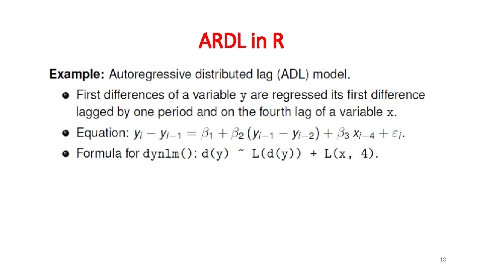
ARDL in R 18

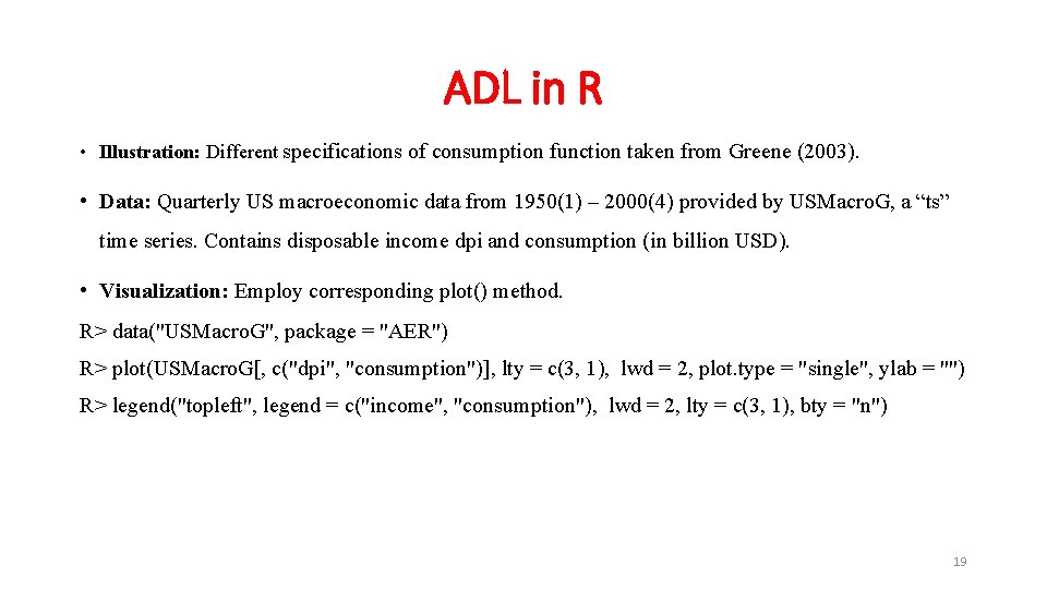
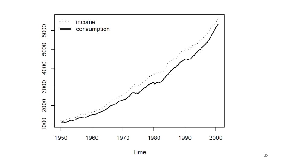
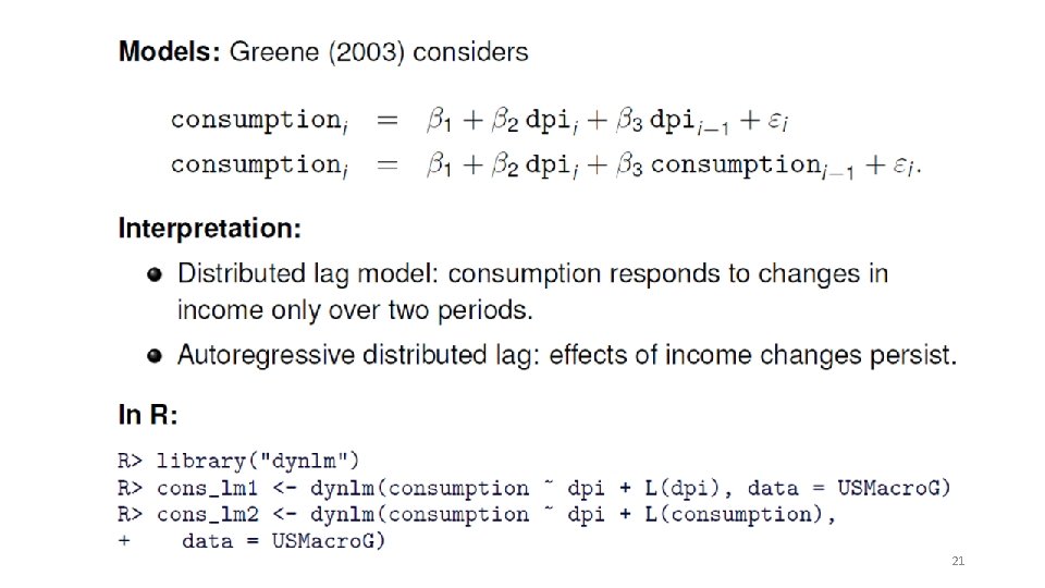
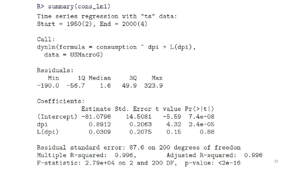
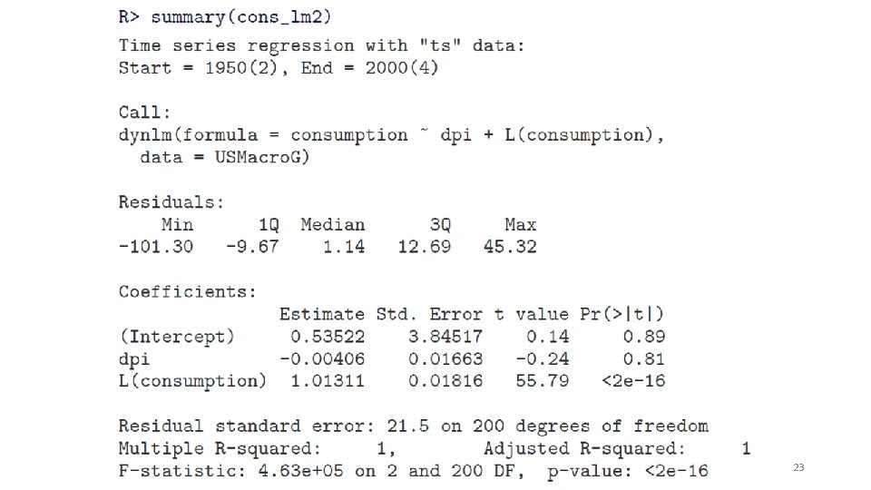
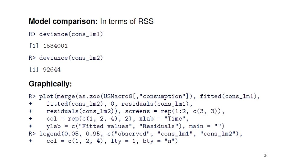
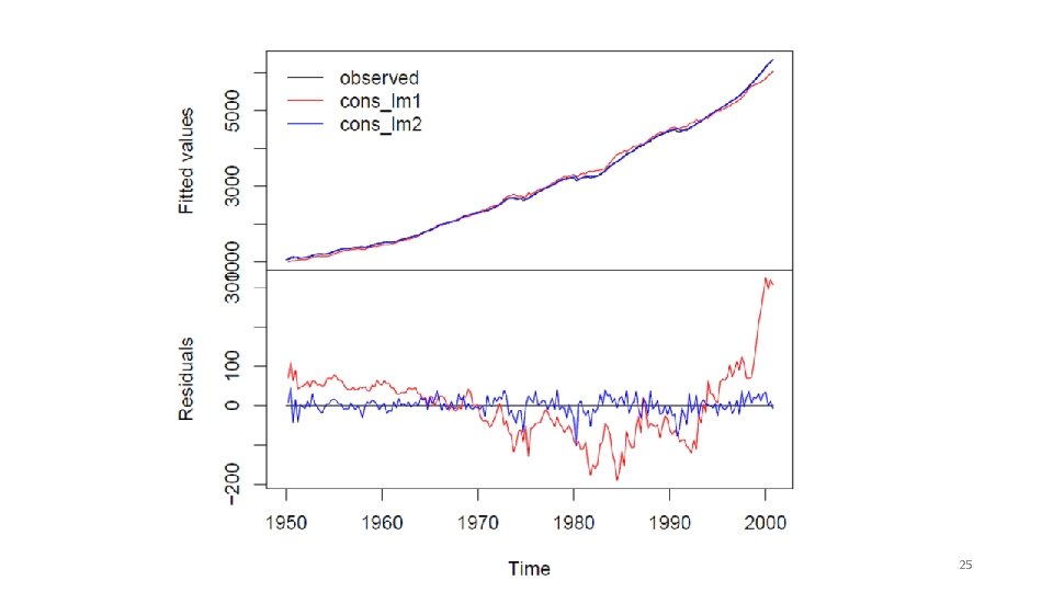
ADL in R • Illustration: Different specifications of consumption function taken from Greene (2003). • Data: Quarterly US macroeconomic data from 1950(1) – 2000(4) provided by USMacro. G, a “ts” time series. Contains disposable income dpi and consumption (in billion USD). • Visualization: Employ corresponding plot() method. R> data("USMacro. G", package = "AER") R> plot(USMacro. G[, c("dpi", "consumption")], lty = c(3, 1), lwd = 2, plot. type = "single", ylab = "") R> legend("topleft", legend = c("income", "consumption"), lwd = 2, lty = c(3, 1), bty = "n") 19

20

21

22

23

24

25

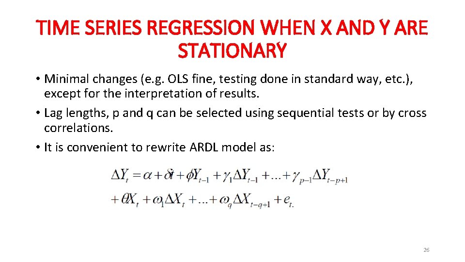
TIME SERIES REGRESSION WHEN X AND Y ARE STATIONARY • Minimal changes (e. g. OLS fine, testing done in standard way, etc. ), except for the interpretation of results. • Lag lengths, p and q can be selected using sequential tests or by cross correlations. • It is convenient to rewrite ARDL model as: 26

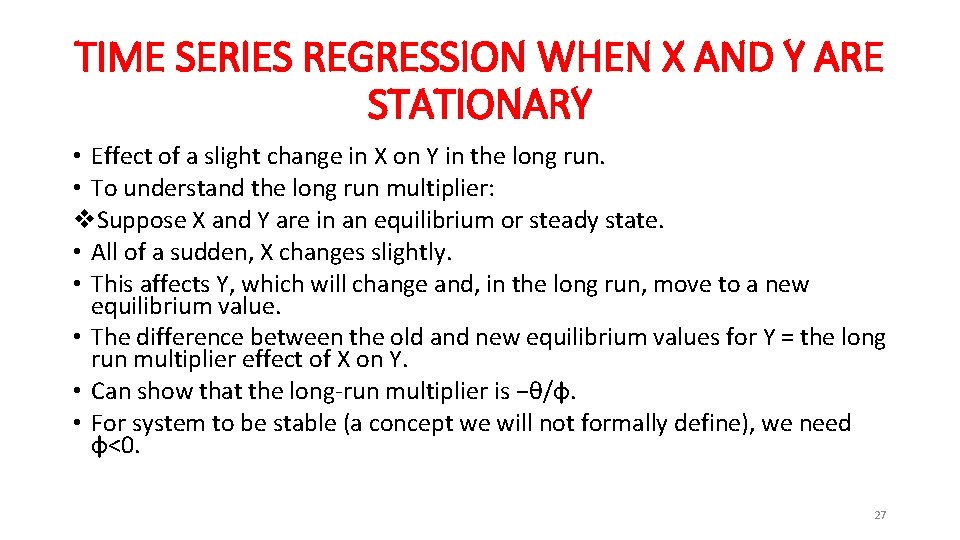
TIME SERIES REGRESSION WHEN X AND Y ARE STATIONARY • Effect of a slight change in X on Y in the long run. • To understand the long run multiplier: v. Suppose X and Y are in an equilibrium or steady state. • All of a sudden, X changes slightly. • This affects Y, which will change and, in the long run, move to a new equilibrium value. • The difference between the old and new equilibrium values for Y = the long run multiplier effect of X on Y. • Can show that the long-run multiplier is −θ/φ. • For system to be stable (a concept we will not formally define), we need φ<0. 27

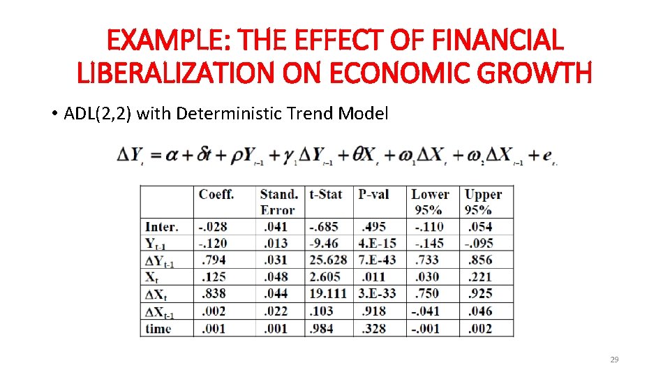
EXAMPLE: THE EFFECT OF FINANCIAL LIBERALIZATION ON ECONOMIC GROWTH • Time series data for 98 quarters for a country • Y = the percentage change in GDP • X = the percentage change in total stock market capitalization • Assume Y and X are stationary 28

EXAMPLE: THE EFFECT OF FINANCIAL LIBERALIZATION ON ECONOMIC GROWTH • ADL(2, 2) with Deterministic Trend Model 29

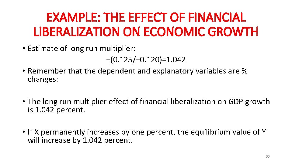
EXAMPLE: THE EFFECT OF FINANCIAL LIBERALIZATION ON ECONOMIC GROWTH • Estimate of long run multiplier: −(0. 125/− 0. 120)=1. 042 • Remember that the dependent and explanatory variables are % changes: • The long run multiplier effect of financial liberalization on GDP growth is 1. 042 percent. • If X permanently increases by one percent, the equilibrium value of Y will increase by 1. 042 percent. 30

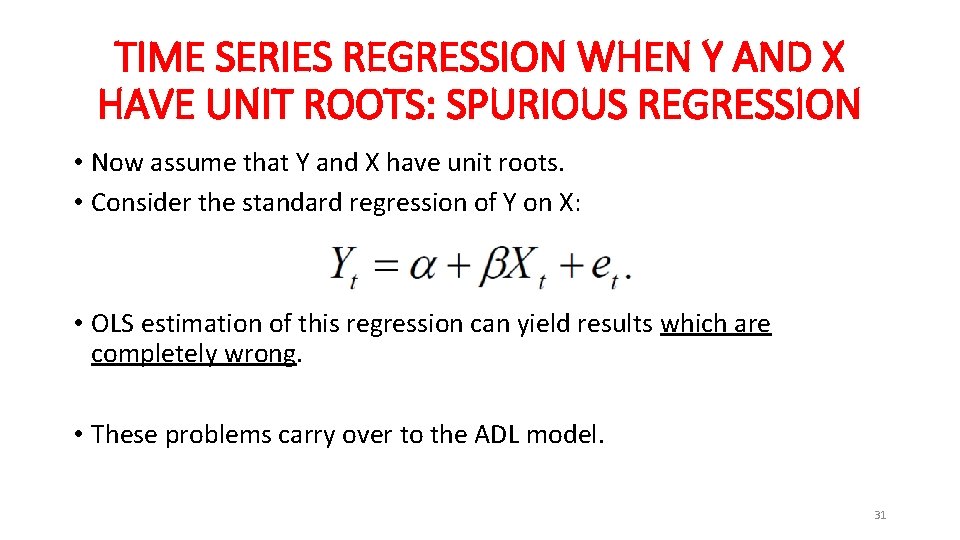
TIME SERIES REGRESSION WHEN Y AND X HAVE UNIT ROOTS: SPURIOUS REGRESSION • Now assume that Y and X have unit roots. • Consider the standard regression of Y on X: • OLS estimation of this regression can yield results which are completely wrong. • These problems carry over to the ADL model. 31

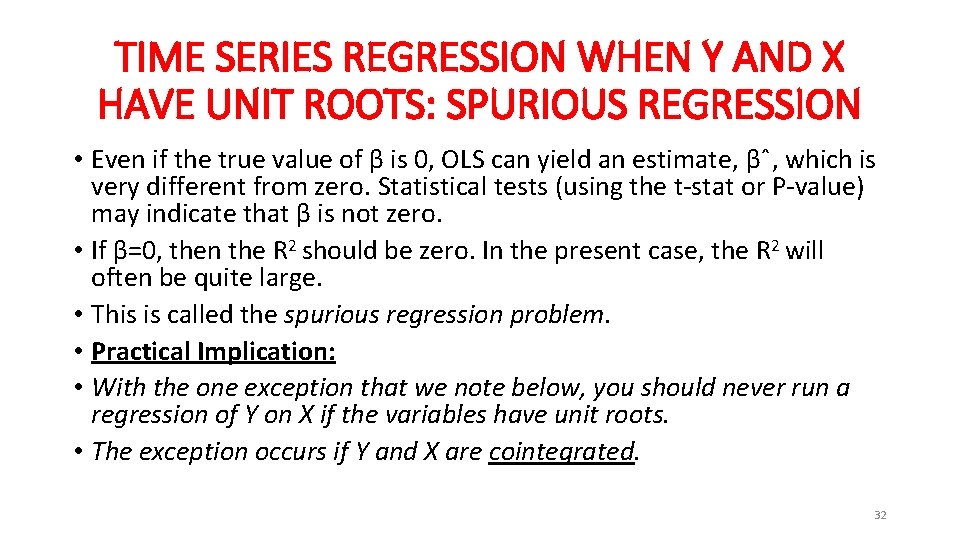
TIME SERIES REGRESSION WHEN Y AND X HAVE UNIT ROOTS: SPURIOUS REGRESSION • Even if the true value of β is 0, OLS can yield an estimate, βˆ, which is very different from zero. Statistical tests (using the t-stat or P-value) may indicate that β is not zero. • If β=0, then the R 2 should be zero. In the present case, the R 2 will often be quite large. • This is called the spurious regression problem. • Practical Implication: • With the one exception that we note below, you should never run a regression of Y on X if the variables have unit roots. • The exception occurs if Y and X are cointegrated. 32

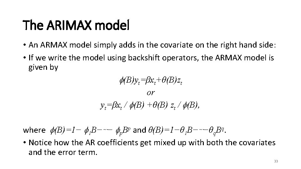
The ARIMAX model • An ARMAX model simply adds in the covariate on the right hand side: • If we write the model using backshift operators, the ARMAX model is given by (B)yt=βxt+θ(B)zt or yt=βxt / (B) +θ(B) zt / (B), where (B)=1− 1 B−⋯− p. Bp and θ(B)=1−θ 1 B−⋯−θq. Bq. • Notice how the AR coefficients get mixed up with both the covariates and the error term. 33

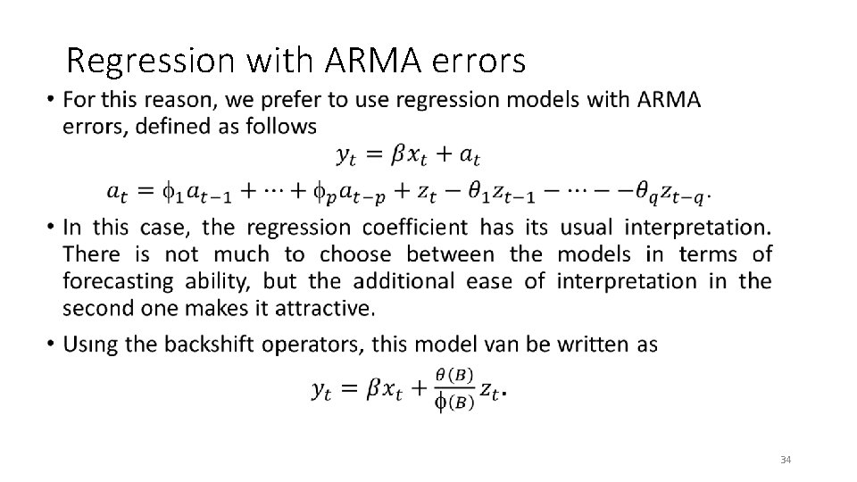
Regression with ARMA errors • 34

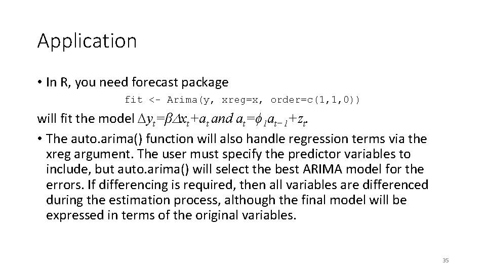
Application • In R, you need forecast package fit <- Arima(y, xreg=x, order=c(1, 1, 0)) will fit the model yt=β xt+at and at=ϕ 1 at− 1+zt. • The auto. arima() function will also handle regression terms via the xreg argument. The user must specify the predictor variables to include, but auto. arima() will select the best ARIMA model for the errors. If differencing is required, then all variables are differenced during the estimation process, although the final model will be expressed in terms of the original variables. 35

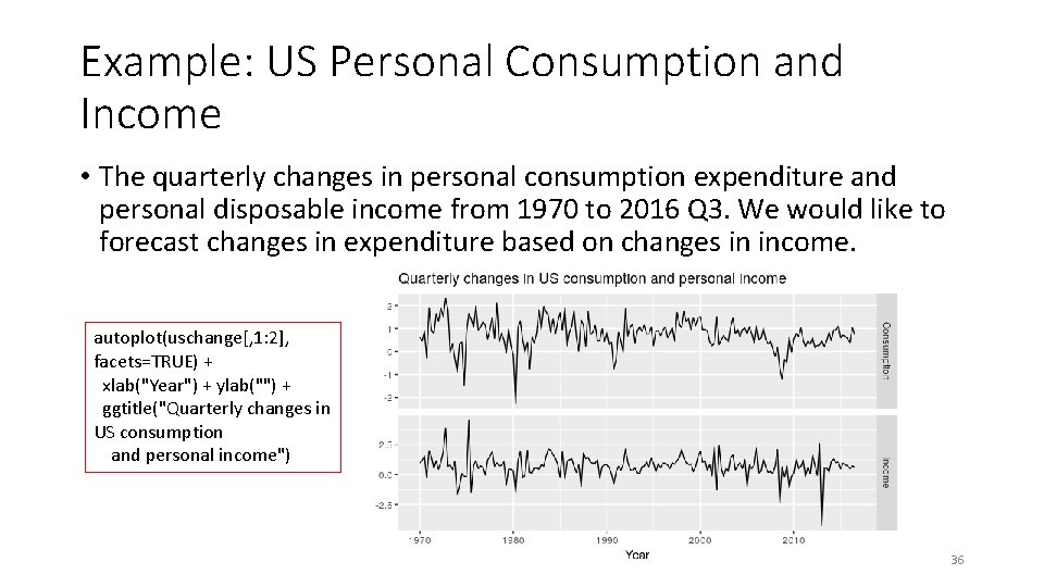
Example: US Personal Consumption and Income • The quarterly changes in personal consumption expenditure and personal disposable income from 1970 to 2016 Q 3. We would like to forecast changes in expenditure based on changes in income. autoplot(uschange[, 1: 2], facets=TRUE) + xlab("Year") + ylab("") + ggtitle("Quarterly changes in US consumption and personal income") 36

(fit <- auto. arima(uschange[, "Consumption"], xreg=uschange[, "Income"])) #> Series: uschange[, "Consumption"] #> Regression with ARIMA(1, 0, 2) errors #> #> Coefficients: #> ar 1 ma 2 intercept xreg #> 0. 692 -0. 576 0. 198 0. 599 0. 203 #> s. e. 0. 116 0. 130 0. 076 0. 088 0. 046 #> #> sigma^2 estimated as 0. 322: #> AIC=325. 9 AICc=326. 4 log likelihood=-156. 9 BIC=345. 3 • The fitted model is yt =0. 599+0. 203 xt+ηt, ηt=0. 692ηt− 1+εt− 0. 576εt− 1+0. 198εt− 2, εt∼NID(0, 0. 322). 37

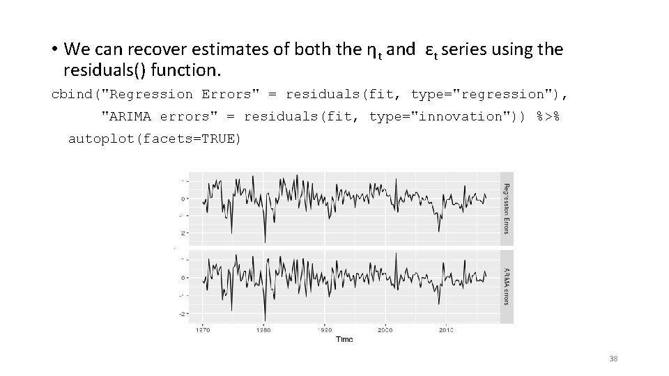
• We can recover estimates of both the ηt and εt series using the residuals() function. cbind("Regression Errors" = residuals(fit, type="regression"), "ARIMA errors" = residuals(fit, type="innovation")) %>% autoplot(facets=TRUE) 38

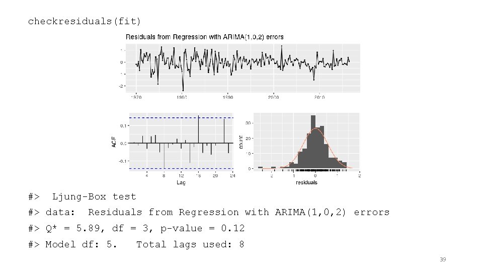
checkresiduals(fit) #> Ljung-Box test #> data: Residuals from Regression with ARIMA(1, 0, 2) errors #> Q* = 5. 89, df = 3, p-value = 0. 12 #> Model df: 5. Total lags used: 8 39

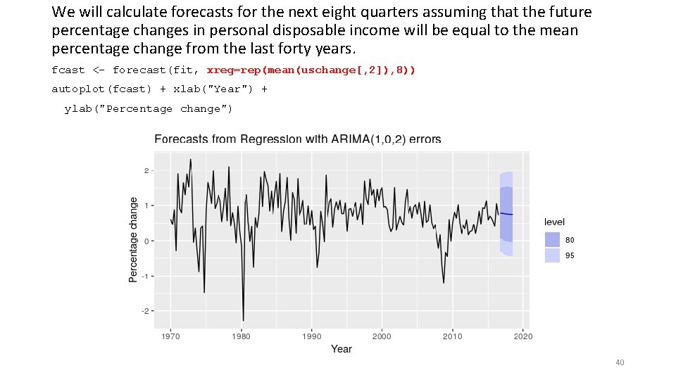
We will calculate forecasts for the next eight quarters assuming that the future percentage changes in personal disposable income will be equal to the mean percentage change from the last forty years. fcast <- forecast(fit, xreg=rep(mean(uschange[, 2]), 8)) autoplot(fcast) + xlab("Year") + ylab("Percentage change") 40

• You can also use TSA or dynlm packages in R. 41

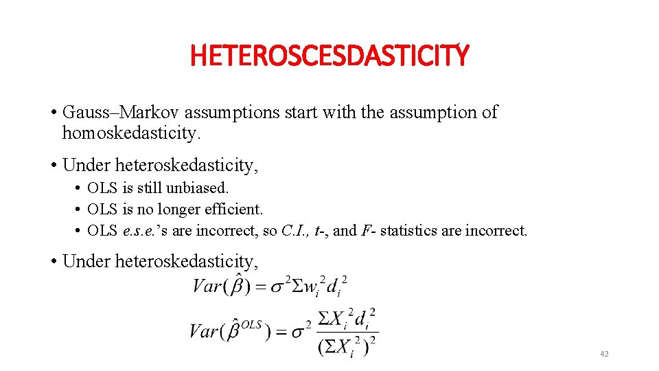
HETEROSCESDASTICITY • Gauss–Markov assumptions start with the assumption of homoskedasticity. • Under heteroskedasticity, • OLS is still unbiased. • OLS is no longer efficient. • OLS e. s. e. ’s are incorrect, so C. I. , t-, and F- statistics are incorrect. • Under heteroskedasticity, 42

HETEROSCESDASTICITY • We can use squared residuals to test for heteroskedasticity. • In the White test, we regress the squared residuals against all explanators, squares of explanators, and interactions of explanators. The n. R 2 of the auxilliary equation is asymptotically distributed Chisquared. • The Breusch–Pagan test is similar, but the we need to choose the explanators for the auxilliary equation. 43

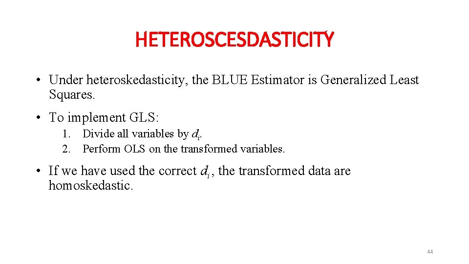
HETEROSCESDASTICITY • Under heteroskedasticity, the BLUE Estimator is Generalized Least Squares. • To implement GLS: 1. Divide all variables by di. 2. Perform OLS on the transformed variables. • If we have used the correct di , the transformed data are homoskedastic. 44

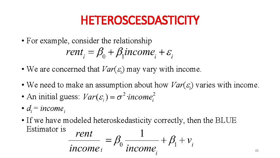
HETEROSCESDASTICITY • For example, consider the relationship • We are concerned that Var( i) may vary with income. • We need to make an assumption about how Var( i) varies with income. • An initial guess: • di = incomei • If we have modeled heteroskedasticity correctly, then the BLUE Estimator is 45

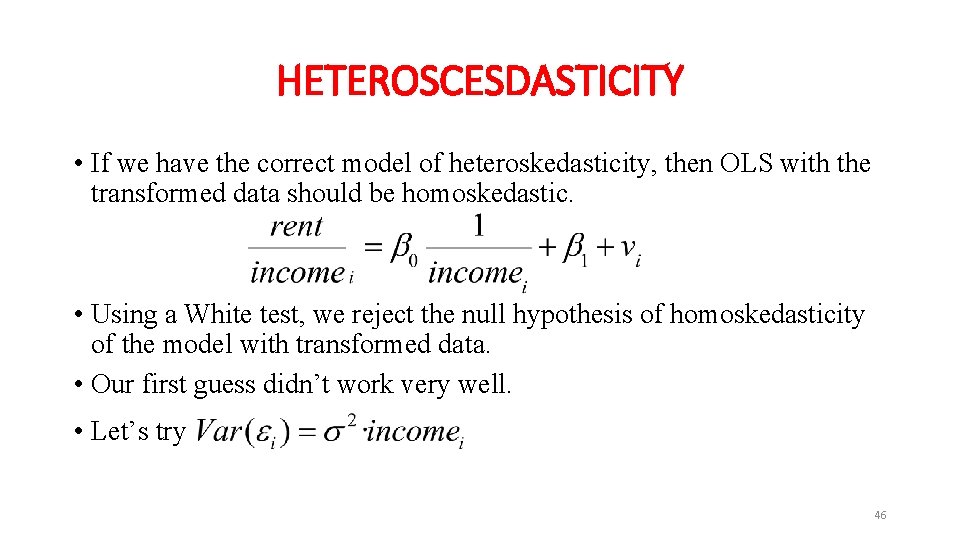
HETEROSCESDASTICITY • If we have the correct model of heteroskedasticity, then OLS with the transformed data should be homoskedastic. • Using a White test, we reject the null hypothesis of homoskedasticity of the model with transformed data. • Our first guess didn’t work very well. • Let’s try 46

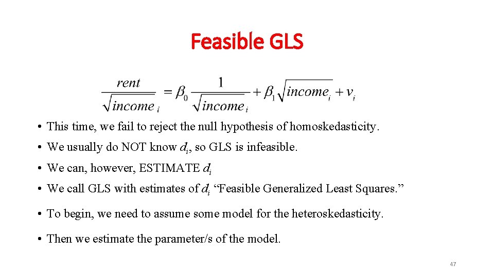
Feasible GLS • This time, we fail to reject the null hypothesis of homoskedasticity. • We usually do NOT know di, so GLS is infeasible. • We can, however, ESTIMATE di • We call GLS with estimates of di “Feasible Generalized Least Squares. ” • To begin, we need to assume some model for the heteroskedasticity. • Then we estimate the parameter/s of the model. 47

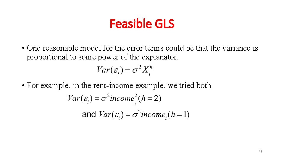
Feasible GLS • One reasonable model for the error terms could be that the variance is proportional to some power of the explanator. • For example, in the rent-income example, we tried both 48

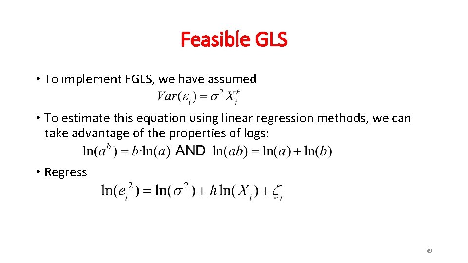
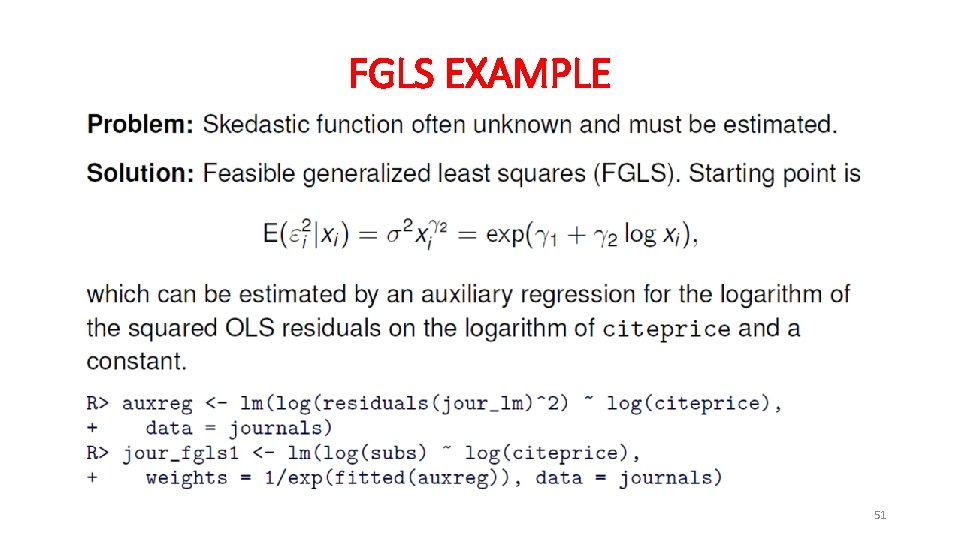
Feasible GLS • To implement FGLS, we have assumed • To estimate this equation using linear regression methods, we can take advantage of the properties of logs: • Regress 49

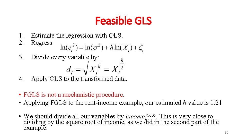
Feasible GLS 1. 2. Estimate the regression with OLS. Regress 3. Divide every variable by: 4. Apply OLS to the transformed data. • FGLS is not a mechanistic procedure. • Applying FGLS to the rent-income example, our estimated h value is 1. 21 • We should divide all our variables by incomei 0. 605. This is very close to dividing by the square root of income, as we did in the second part of the example. 50

FGLS EXAMPLE 51

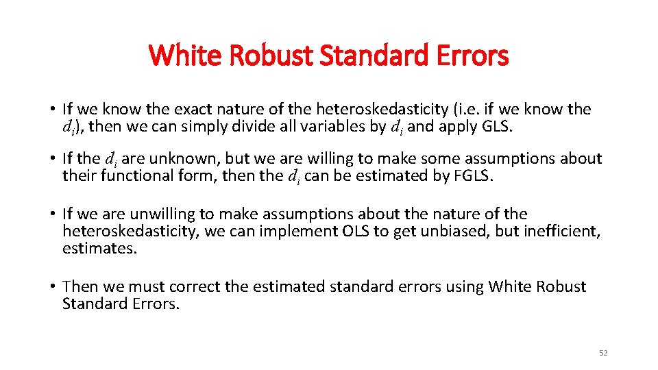
White Robust Standard Errors • If we know the exact nature of the heteroskedasticity (i. e. if we know the di), then we can simply divide all variables by di and apply GLS. • If the di are unknown, but we are willing to make some assumptions about their functional form, then the di can be estimated by FGLS. • If we are unwilling to make assumptions about the nature of the heteroskedasticity, we can implement OLS to get unbiased, but inefficient, estimates. • Then we must correct the estimated standard errors using White Robust Standard Errors. 52

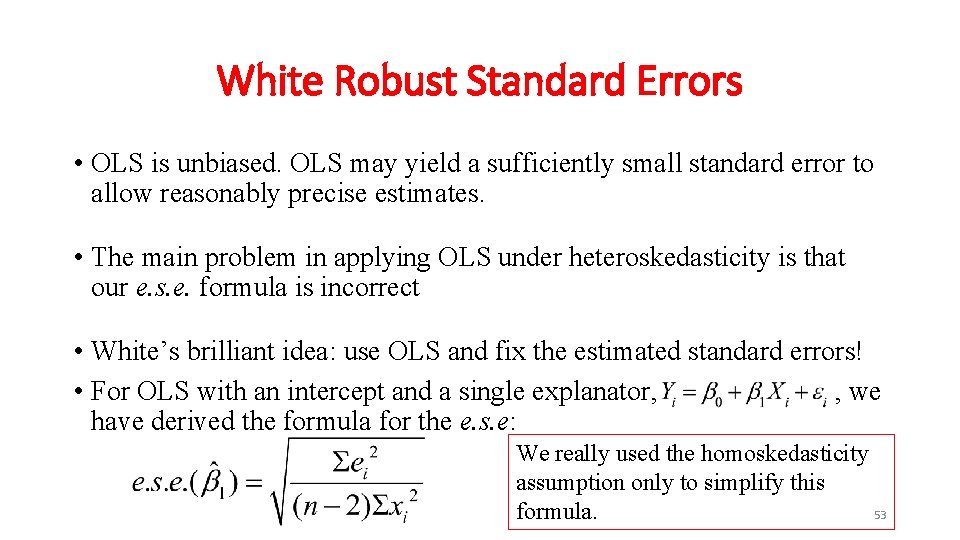
White Robust Standard Errors • OLS is unbiased. OLS may yield a sufficiently small standard error to allow reasonably precise estimates. • The main problem in applying OLS under heteroskedasticity is that our e. s. e. formula is incorrect • White’s brilliant idea: use OLS and fix the estimated standard errors! • For OLS with an intercept and a single explanator, , we have derived the formula for the e. s. e: We really used the homoskedasticity assumption only to simplify this formula. 53

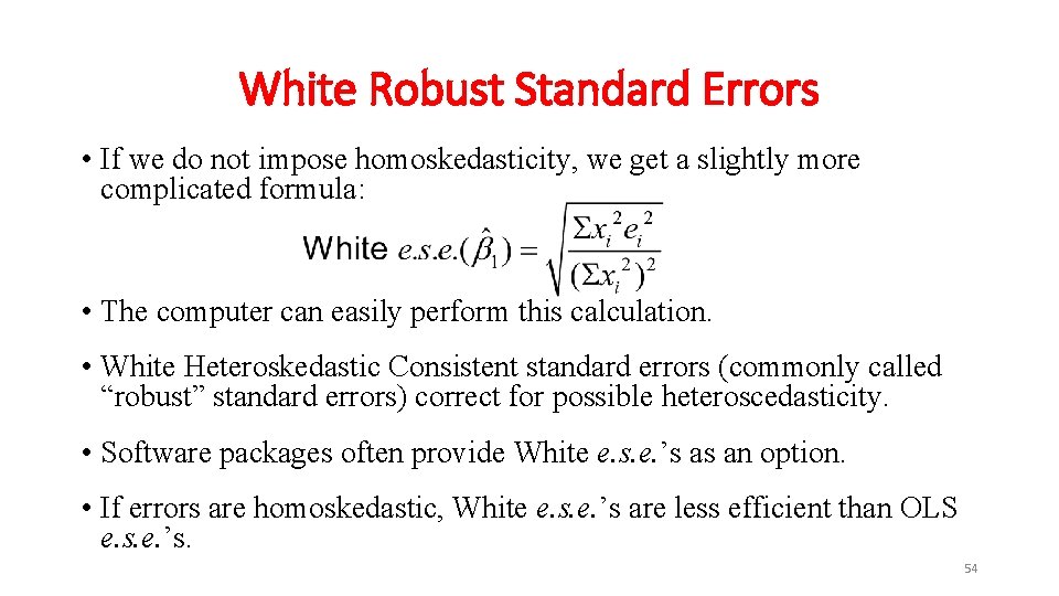
White Robust Standard Errors • If we do not impose homoskedasticity, we get a slightly more complicated formula: • The computer can easily perform this calculation. • White Heteroskedastic Consistent standard errors (commonly called “robust” standard errors) correct for possible heteroscedasticity. • Software packages often provide White e. s. e. ’s as an option. • If errors are homoskedastic, White e. s. e. ’s are less efficient than OLS e. s. e. ’s. 54

White Robust Standard Errors • Applying White estimated standard errors is a very easy fix for possible heteroskedasticity. • Some analysts simply use White e. s. e. ’s routinely. • This fix comes with a cost in efficiency: • OLS is not BLUE under heteroskedasticity. • White e. s. e. ’s are inefficient under homoskedasticity. 55

HETEROSCESDASTICITY • Heteroskedasticity is not, in practice, a burdensome complication. • Tests to detect heteroskedasticity • White tests • Breusch–Pagan tests • Goldfeld–Quandt tests 56

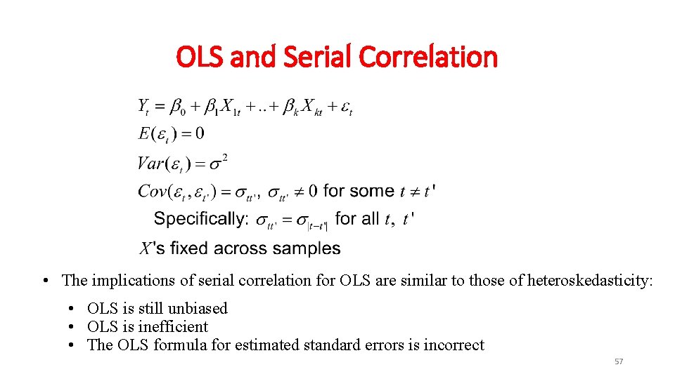
OLS and Serial Correlation • The implications of serial correlation for OLS are similar to those of heteroskedasticity: • OLS is still unbiased • OLS is inefficient • The OLS formula for estimated standard errors is incorrect 57

OLS and Serial Correlation • As with heteroskedasticity, we have two choices: 1. We can transform the data so that the Gauss–Markov conditions are met, and OLS is BLUE; OR 2. We can disregard efficiency, apply OLS anyway, and “fix” our formula for estimated standard errors. • We will first consider the strategy of “fixing” the estimated standard errors from OLS. • Newey–West Serial Correlation Consistent Standard Errors 58

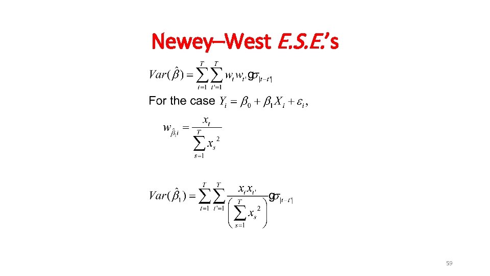
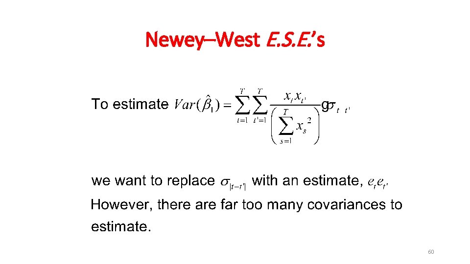
Newey–West E. S. E. ’s 59

Newey–West E. S. E. ’s 60

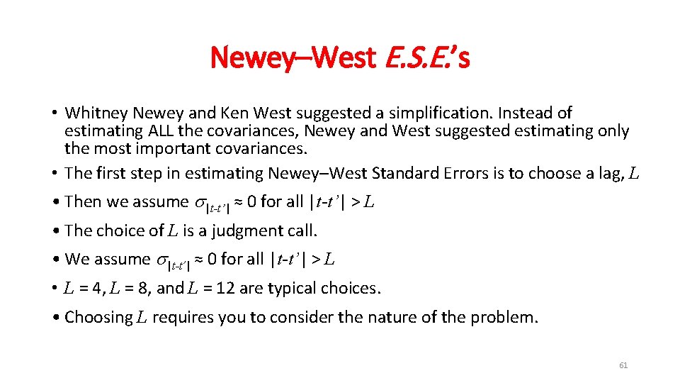
Newey–West E. S. E. ’s • Whitney Newey and Ken West suggested a simplification. Instead of estimating ALL the covariances, Newey and West suggested estimating only the most important covariances. • The first step in estimating Newey–West Standard Errors is to choose a lag, L • Then we assume s|t-t’| ≈ 0 for all |t-t’| > L • The choice of L is a judgment call. • We assume s|t-t’| ≈ 0 for all |t-t’| > L • L = 4, L = 8, and L = 12 are typical choices. • Choosing L requires you to consider the nature of the problem. 61

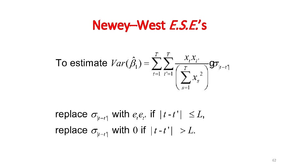
Newey–West E. S. E. ’s 62

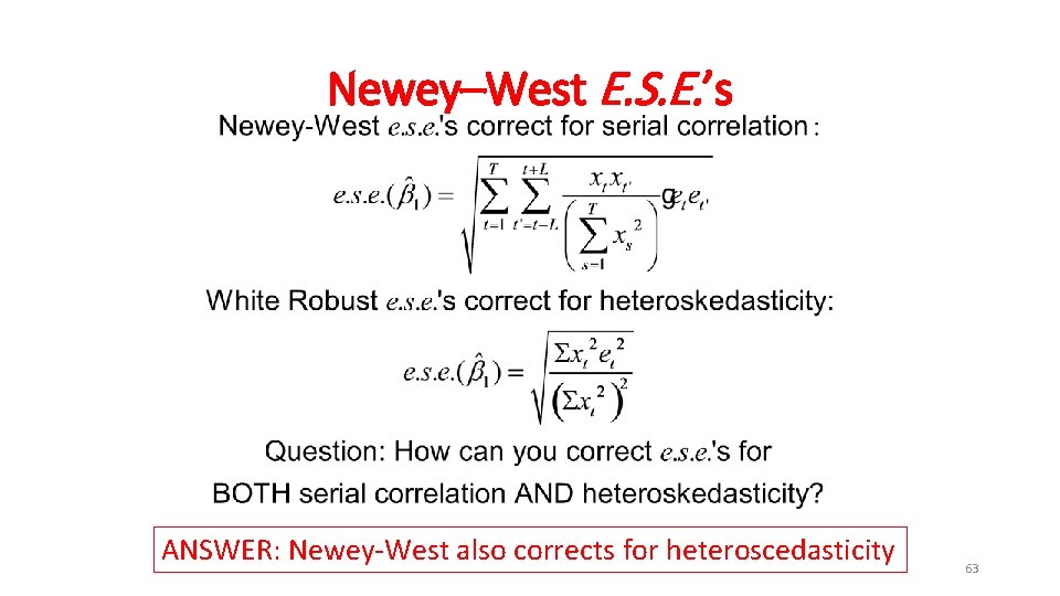
Newey–West E. S. E. ’s ANSWER: Newey-West also corrects for heteroscedasticity 63

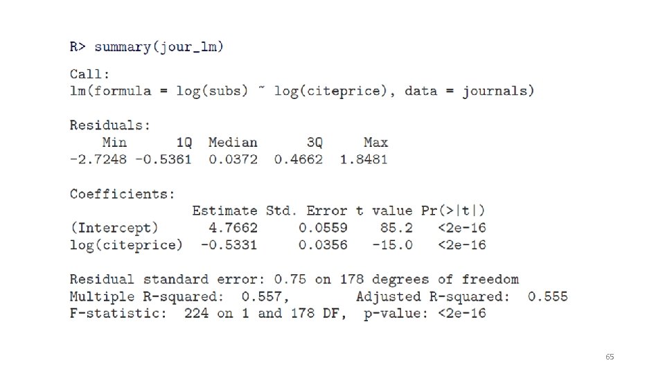
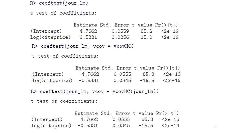
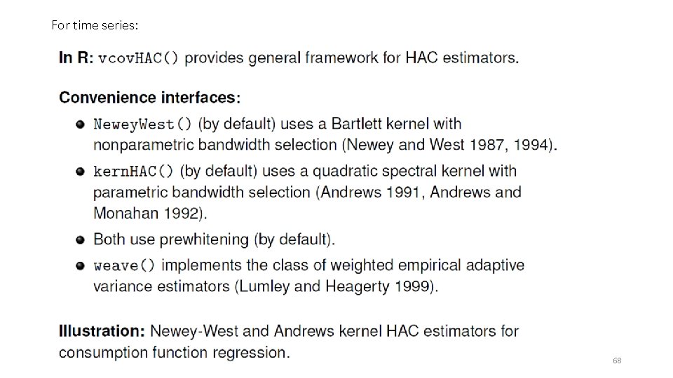
Robust Standard Errors and Tests • Heteroskedasticity consistent (HC) and heteroscedasticity and autocorrelation consistent (HAC) covariance matrix estimators • Package sandwich (automatically loaded with AER) provides HC and HAC counterparts of vcov(): vcov. HC() and vcov. HAC() 64

65

66

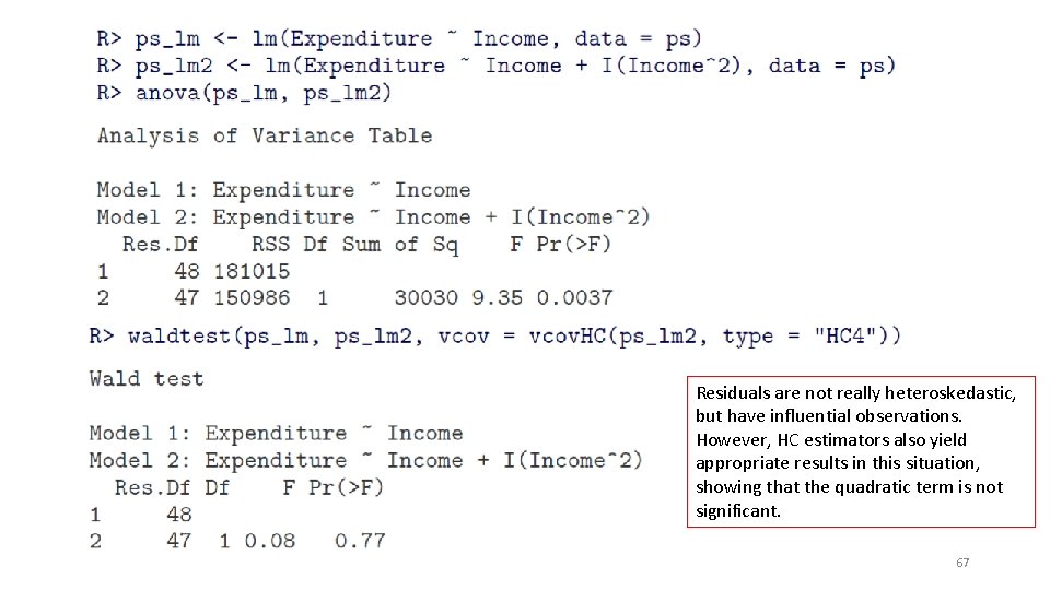
Residuals are not really heteroskedastic, but have influential observations. However, HC estimators also yield appropriate results in this situation, showing that the quadratic term is not significant. 67

For time series: 68